1. Homeowners Insurance Market in Texas with Catastrophic Effects:
Market Competition, Supply and Demand
May 13, 2013
Jingting Yi
Department of Economics
University of California, Berkeley
Berkeley, CA 94720
jyi_90715@berkeley.edu
Under the supervision of Professor Ben Handel
ABSTRACT
Because of the catastrophic effects of natural disasters, the homeowners insurance market often displays different profit and loss patterns from those of other lines of property and casualty insurance. Using the homeowners insurance data in Texas from 1995 to 2011, along with the catastrophe data and macroeconomic in same period, this paper evaluates the market competition, demand and supply of this market. The homeowners insurance market in Texas is moderately competitive, with decent profitability and some entries exits each year. On the supply side, insurance companies adapt to excessive losses due to catastrophic risks by raising their premiums, while some even go insolvent and leave the market. On the demand side, an increasing number of people purchase homeowners insurance policies through the time period of interest. This trend is driven by the changes in average premiums, population and house prices, etc.
____________________________________________________________________________
Acknowledgements: I would like to sincerely thank Professor Ben Handel for his supervision and support throughout my research, from whose inspiring advices I have learned a lot in both my research topic and the general research process. I would also like to thank Tapio Boles, Senior Consultant at Towers Watson and Alen Gong, Actuarial Analyst in AAA NCNU Insurance Exchange for helping me with data sources insurance knowledge.

2. 1. Introduction
In most of the lines in property and casualty insurance, such as automobiles, workers’ compensation and general liability, the insurers undertake a large amount of independent risks and the risk pattern is similar across different years. Therefore, except for significant macroeconomic or policy changes, one would expect the price of insurance to be fairly stable or following a steady trend.
However, the case is very different for homeowners insurance pricing, in which catastrophes play a very important role, as insurance companies are faced with more uncertainties, because of a variety of reasons.
First, in contrast to automobile insurance, in which the frequency of claims of the insured cars is rather stable in different years and thus the loss trend by year is rather smooth, homeowners insurance faces a much more dramatic loss pattern. There may be no claims at all in one year, but many gigantic claims in another. Some insurance companies even go insolvent and stop writing business in some states because of severe catastrophes.
Also, because of the relatively low probability a catastrophic event, it is really hard to fully learn and model the risks. All that the insurance companies can do is to learn from the past catastrophic events and predict the frequency and severity of future events. However, the modeling of catastrophic risks has only developed for tens of years, so the data available are not sufficient for performing accurate predictions. Therefore, insurance companies are still on their way to develop the best modeling system and pricing strategy to capture the risks. In addition, there are a lot of other factors influencing the likelihood catastrophic event,

3. such as how global warming influences the tropical storms1 and how natural gas drilling influences the earthquake2. Thus the past data, even if they accurately reflect frequency and severity of the catastrophic events, may not well predict the behaviors of future catastrophes, making catastrophe insurance pricing even harder. Therefore, when new catastrophes occur, it is very likely for insurance companies to adjust their premium rate accordingly.
Furthermore, in the catastrophe insurance market, the demand of insureds also tends to be biased. Howard Kunreuther has found that ‘Individuals are only myopic and hence only take into account the potential benefits from such (insurance) investments over the next year or two’. Therefore, it’s very likely that the occurrence of a catastrophic event will encourage more people to buy insurance and vice versa.
One last observation of the catastrophe insurance market is that, it does not seem to be affected by the macroeconomic condition same ways as other markets. For instance, in the years following Great Recession, while home prices were falling, insurance premiums were on the rise3. This might be because the rebuilding cost, which is a big factor that insurers care about in pricing homeowner insurance, actually rose instead of falling during those years. However, the macroeconomic changes affect people’s demand for homeowners insurance policies in quite a similar way as for other goods. This inconsistency of the changes in demand and supply might generate interesting changes the price of catastrophe insurance.
In this paper, I will conduct an empirical and econometric analysis on the market
1 Discussed in Knutson (2013), “Global Warming and Hurricanes”.
2 Discussed in Carlton, “Drilling might be culprit behind Texas earthquakes”.
3 Discussed in Terhune and Andriotis (2011). “While Home Prices May Be Falling, Insurance Premiums Are on the Rise”.

4. competition, demand and supply in the homeowners insurance market Texas, taking into consideration the catastrophic risks. Section 2 describes data sources and variables used in this paper. Section 3 describes the general features of this market by looking at premiums, losses, entries, exits and market concentration to obtain some insight of the competition this market. Section 4 focuses on the supply side of market, where I conduct several regression analyses to assess the impacts of loss ratios, catastrophes and house prices on average premiums. Section 5 focuses on the demand side of market, exploring into possible factors that drive people to buy more insurance policies, such as average premiums, losses per policy, catastrophes, populations and house prices.
2. Data Sources
The first set of data used in this paper is the annual Homeowners section of Property and Casualty Insurance Experience by Carriers from 1995 to 2011 published Texas Department of Insurance. Since different states in the U.S. are exposed to different kinds and scales of catastrophes, I believe it would be more consist to focus on one state to study the behaviors of the homeowners insurance market. Texas is chosen because it has a relatively large market size, it is exposed to severe catastrophe risks (mainly hurricanes and tropical storms) and it has been one of the states with the most expensive homeowner insurance for many years. From this data set, I compile a list of all the insurance companies that have written homeowner insurance in those 17 years and matched them with their Direct Premiums Earned and Direct Losses Incurred4 for each year. I then sum up the data of each
4 Direct Premiums Earned and Losses Incurred are chosen instead of Written Paid to be consistent with loss the ratio calculation adopted by Texas Department of Insurance.

5. year as Total Premiums and Losses so that I can further study the premium and loss trends. I also calculate some other relevant variables from the data set such as:
Loss Ratio (t): Total Losses divided by Premiums in year t.
Number of Insurers (t): Number of insurance companies that write homeowner policies in Texas in year t.
Exit (t): For each insurance company that had a presence in Texas homeowner market, I assign a value of 1 if the company wrote policies of homeowner insurance in Texas in year t-1 but stopped writing policies in year t, and 0 otherwise. Summing these values across all the companies gives my total exit of year t.
Entry (t): Number of Companies in year t subtracted by Exit t.
Also the insurance companies in Texas are divided in to 5 categories of organizational forms, Reciprocal, Mutual, Lloyd, Stock and County Mutual. Because Mutual insurance size is relatively small and has a significantly different risk pattern from other types (in the data package it’s a different file) so we exclude this part. We also exclude Stock5. We use the rest of three categories to see whether insurances companies of different structures behave differently in catastrophe insurance pricing.
Reciprocal Premiums and Losses: Total premiums and losses if the company is Reciprocal.
Mutual Premiums and Losses: Total premiums and losses if the company has a Mutual insurance structure.
Lloyd’s Premiums and Losses: Total premiums and losses if the company has a
5 For a detailed review of the effect of organizational form on insurer performance see Born, Gentry, Viscusi, and
Zeckhauser (1998).

6. Lloyd’s insurance structure.
The second set of data set used in this paper is the catastrophe data in Texas as well the Atlantic Basin. The catastrophes I include in this discussion are mainly hurricanes, tropical storms and tornadoes, since these are the natural disasters that happen most frequently and cause the largest losses. In Texas, earthquake is covered separately from homeowner insurance and Texas is not faced with severe risks of earthquakes, therefore earthquake events are not included in my discussion. I also include the number of hurricanes and tropical storms in the North Atlantic because I’m interested in whether the occurrence of a large catastrophe nearby can impact the insurance market in Texas. A further description of the variables used is as follows:
TXCat (t): This is number of catastrophes in Texas in year t that caused over $10 million loss, obtained from the ISO (Insurance Services Office) Catastrophe report. The catastrophes include hurricanes, wind and thunderstorms tropical storms.
UnexpCat (t): This is obtained by subtracting the average number of catastrophes throughout the years of interest from number catastrophes in year t6.
Blockbuster7 (t): This is a dummy variable. The value is 1 if there a catastrophe in year t that caused over $1 billion loss and 0 otherwise.
ATCat (t): This is the number of large catastrophes in North Atlantic that caused damages of over $1 billion less such events in Texas year t.
The third set of data used in this paper includes the average premiums of homeowners insurance in Texas from 1995 to 2011, obtained from the Report to Senate Business and
6 Here we use the average in these 17 years as expected number of losses, since it’s best estimate with given data.
7 Term used in Born and Viscusi (2006)

7. Commerce Committee of Texas Homeowner Insurance. With that data, I also calculate the number of homeowner policies and Loss Per Policy each year.
Policy Counts (t): Total Premiums in year t divided by Average Premium t.
Loss Per Policy (t): Total Losses in year t divided by Policy Counts t.
The percentage changes of Average Premium, Loss per Policy and Counts are also calculated and denoted as Rate Change, Average Loss Change and Policy Count Change.
The last set data is regarding the macroeconomic conditions of US in 1995-2011, including National Housing Price Index obtained from the Federal Reserve Economic Data and Texas Population, obtained from the Census Bureau. The percentage changes are also calculated and denoted as House Price Change and Population Change.
3. General Features of Homeowners Insurance Market in Texas and Market Competition
3.1 Premiums, Losses, Loss Ratios
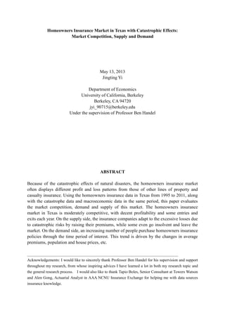
To start with, I look at the general performances of Texas’s insurance companies throughout these years. Figure 1 shows that premiums have been growing steadily but losses have been displayed in a more volatile pattern.

8. Figure 1 Total Premiums and Losses of Texas Homeowners Insurance, 1995-2011
Figure 2 Loss Ratio of Texas Homeowners Insurance, 1995-2011
Figure 2 shows that loss ratios have also been volatile but averaged at around 60%. Even in the worst years (Year 2001, 2002 and 2008), the loss ratios were only slightly above 1, unlike Florida’s 990.3% loss ratio in 1992. This means that the insurance companies in Texas have generally managed their homeowners risks quite well. In this market, the loss ratio is principal factor, though not the only one, that affects an insurance company’s profitability. Therefore, I would conclude that the loss ratio pattern here shows high profitability of the homeowners insurance market.
-
1,000,000,000
2,000,000,000
3,000,000,000
4,000,000,000
5,000,000,000
6,000,000,000
7,000,000,000
8,000,000,000
1995
1996
1997
1998
1999
2000
2001
2002
2003
2004
2005
2006
2007
2008
2009
2010
2011
Total Premium and Loss
Total Premium
Total Loss
0.00%
20.00%
40.00%
60.00%
80.00%
100.00%
120.00%
140.00%
1995
1996
1997
1998
1999
2000
2001
2002
2003
2004
2005
2006
2007
2008
2009
2010
2011
Loss Ratio

9. 3.2 Market Concentration
To further analyze the competition of this market, I use the market concentration ratios at the 1-firm (CR1), 2-firm (CR2), 4-firm (CR4), 8-firm (CR8) and 20-firm (CR20). A concentration ratio shows the combined market share of insurance companies with highest premiums. For example, CR1 means the market share of top insurer and CR4 means the combined market share of top four insurers. A high concentration ratio the largest companies take up a high percentage of the market share and thus possess great market power. Therefore, it can be a good measure of competition.
In Texas, the market concentration ratios have been rather stable throughout 1995 to 2011, with fluctuations within 10%, possibly due to poor underwriting behaviors of some insurers in years with large catastrophe losses. The premium weighted average is 29.47% for CR1, 41.95% for CR2, 54.29% for CR4, 69.01% CR8, and 86.22% CR20. From these figures, we can see that there is a big market player taking around 30% of the share (State Farm Lloyd’s), but not big enough to function as a monopoly. There are also few big market players in the homeowner insurance Texas, but they do not dominate market either. Moreover, there are many middle-sized insurers that take up a considerable market share. From these traits in the market concentration ratios, I believe that the homeowner insurance market in Texas is moderately competitive.
3.3 Numbers of Companies, Entries and Exits
Another way to assess the market competition is by looking at the change in the number of companies. Low entry and exit barriers serve as a good indicator of competitive market. Therefore, we would expect some companies entering and exiting the market every year for a

10. competitive market. In the insurance market, on one hand, there should be new companies entering the market to respond increasing demand and profitability in the market. On other hand, there should also be insurance companies that fail to cover underwriting risks exiting the market. Also, we would expect that this market has significant barriers in since Texas is exposed to great catastrophe risks and regulations can also serve as an impeding factor. For instance, one way regulators can impose an exit barrier is by requiring an insurer to exit all lines of business in a state if it wishes to exit particular line, such as homeowners or auto insurance.
Figure 3.1 Numbers of Companies in Texas Homeowners Insurance, 1995-2011
Figure 3.2 Numbers of Exits in Texas Homeowners Insurance, 1996-2011
-
50
100
150
200
250
300
350
1995
1996
1997
1998
1999
2000
2001
2002
2003
2004
2005
2006
2007
2008
2009
2010
2011
Number of Companies
-
10
20
30
40
50
1996
1997
1998
1999
2000
2001
2002
2003
2004
2005
2006
2007
2008
2009
2010
2011
Number of Exits

11. Figure 3.3 Numbers of Entries in Texas Homeowners Insurance, 1996-2011
From Figure 3.1, 3.2 and 3.3, we can see that the number of companies have been gradually decreasing throughout the years, from 298 in year 1995 to 220 2011, and each year has a small number of entries and exits. The data pattern shows that the homeowners insurance market is rather competitive given the possible entry and exit barriers. However, it is interesting to see that there have been more exits than entries in general despite the high profitability of this market and the general increasing number of insurers nationwide. This might be related to some insurance companies’ strategies to switch their business low-risk area. In the section 4, we will further conduct a regression analysis on the potential drivers for the numbers of entries and exits.
3.4 Insurances by Organizational Forms: Reciprocal vs. Mutual Lloyd’s
Insurers in Texas studied this paper are categorized into three different groups by organizational forms, Reciprocal, Mutual and Lloyd’s. In a reciprocal insurance exchange each member of the association assumes the risk of other. Profits and losses are shared in direct proportion to how much insurance coverage a member has. A mutual insurance company is owned by the insureds, and places premium dollars that are received into a pool, which is used to pay claims. Lastly Lloyd's is a marketplace where members join together as
-
5
10
15
20
25
30
35
1996
1997
1998
1999
2000
2001
2002
2003
2004
2005
2006
2007
2008
2009
2010
2011
Number of Entries

12. syndicates to insure risk. Here I want to study whether there is a difference among their premium and loss patterns for different structures of the insurance companies.
Figure 4.1 Total Premiums: Reciprocal VS Mutual Lloyd’s
Figure 4.2 Total Losses: Reciprocal VS Mutual Lloyd’s
Figure 4.3 Loss Ratios: Reciprocal VS Mutual Lloyd’s
From the comparisons of premiums, losses and loss ratios in Figure 4.1, 4.2 4.3, we can see that insurances companies with a Lloyd’s structure take up the majority of business in Texas, followed by Reciprocal then Mutual. Also, the Lloyd’s insurance companies experienced a more drastic change in both premiums and losses, but its loss ratio trend is the most stable among three. In general, all three groups follow a similar to the loss trend of all insurance companies. The discrepancies among them might result from
$0
$1,000,000,000
$2,000,000,000
$3,000,000,000
$4,000,000,000
1995
1996
1997
1998
1999
2000
2001
2002
2003
2004
2005
2006
2007
2008
2009
2010
2011
Total Premiums
Reciprocal
Mutual
Lloyds
$0
$1,000,000,000
$2,000,000,000
$3,000,000,000
$4,000,000,000
$5,000,000,000
1995
1996
1997
1998
1999
2000
2001
2002
2003
2004
2005
2006
2007
2008
2009
2010
2011
Total Losses
Reciprocal
Mutual
Lloyds
0.00%
50.00%
100.00%
150.00%
200.00%
250.00%
1995
1996
1997
1998
1999
2000
2001
2002
2003
2004
2005
2006
2007
2008
2009
2010
2011
Loss Ratio
Reciprocal
Mutual
Lloyds

13. the scales of business.
4. Homeowners Insurance in Texas: Supply
4.1 The Effect of Loss Ratio and Housing Price on Average Premium
In this section, I want to study how different factors can affect the pricing of homeowners insurance. To start with, I look at the average premium trend of Texas compared to those of some other states and countrywide. Figure 4.1 shows how the average premiums have developed from 1995 to 2008 in the some states and countrywide. Though there are some caveats in the comparison8, we can still see that Texas’s rate for homeowner insurance has always been among the highest and significantly higher than nationwide average.
Figure 5.1 Homeowners: Comparison of Average Premiums (Redraw later) 8 Texas policy forms are different than the single form primarily used in the other states, and for this reason NAIC states that Texas data is not comparable to other states; Texas data includes the coastal wind risk written by its insurer of last resort (Texas Windstorm Insurance Association) while Florida data does not include its coastal wind risk (written by Citizens Property Insurance Corporation, its insurer of last resort). For this reason NAIC states that Florida’s premium cost is significantly under-reported.
0
200
400
600
800
1000
1200
1400
1600
1800
1995
1996
1997
1998
1999
2000
2001
2002
2003
2004
2005
2006
2007
2008
Average Premium Comparison
Countrywide
Texas
Florida
Louisiana
Oklahoma
California
New York

14. Figure 5.2 Average Premiums of Texas Homeowner Insurance, 1995-2011
Then, looking closely at the average premium trend in Texas in Figure 5.2, we can see an interesting pattern: the average premium grew steadily and slowly from 1995 to 2001 then from 2001 to 2002, it suddenly jumped 951 1232 (29.55%); then after 2002, the trend flattened again and stayed rather still for some years until 2008; from 2008 to 2011, the average premium increased by a noticeable amount each year. One possible explanation for the sudden and significant rate change in 2002 might be related to the policy changes of Texas homeowners insurance. In the early 2000s, comprehensive homeowners policies (called HO-B policies) are no longer offered by most insurers and are priced out of reach for many homeowners. Instead, insurers have parceled out protections, selling some formerly standard coverages to homeowners at an additional cost9. Therefore, a saying of ‘paying more for less’ stemmed from this change. Another interpretation is that the high loss ratio in year 2011 after many years of low loss ratios made insurers think that they did not accurately model the catastrophic risks in Texas and previous premiums was too low to cover the losses. Therefore, they need to raise the premium both have sufficient amount of money cover future losses and to make up for the excessive losses of the previous years. If this hypothesis
9 For more details, see “Overview of Texas Homeowners Policy Coverage”.
791
812
840
865
860
877
951
1232
1249
1244
1222
1215
1251
1272
1332
1382
1412
0
200
400
600
800
1000
1200
1400
1600
1995
1996
1997
1998
1999
2000
2001
2002
2003
2004
2005
2006
2007
2008
2009
2010
2011
Average Premium

15. is correct, loss ratios should have a positive effect on the rate change in the following year.
In addition, the macroeconomic conditions can also be a factor that influences insurance rate. Here I want to look at whether the house price change has an effect on insurance rate change to gain some insight into how insurance companies respond macroeconomic changes.
Therefore, the regression model here is 푹풂풕풆푪퐡풂풏품풆풕=훃ퟎ+훃ퟏ푳풐풔풔푹풂풕풊풐풕−ퟏ+훃ퟐ푯풐풖풔풆푷풓풊풄풆푪풉풂풏품풆풕
From Table 1, we can see that the regression coefficient for Loss Ratio is statistically significant at 5% significance level so we can reject the null and conclude that the rate change is associated the loss ratio in previous year. The estimated coefficient is 0.13419, indicating that 1% change in loss ratio will incur 0.13419% rate change. The ratio has a positive effect on the insurance pricing, which complies with our hypothesis.
However, the regression coefficient for House Price Change is not statistically significant so we cannot reject the null. This indicates that rate change is not associated with the house price change. In Figure 6, we can see that in years following the Great Recession (year 2008), housing price significantly dropped at around 5% annual rate but insurance still increased at around 5% annual rate. Thus, my data show that the housing price is not a significant driver for the premium rate change. One explanation is that property insurance is more associated with rebuilding cost than housing price, and costs have not dropped since the Financial Crisis. Also, I notice that the validity of this result is subject the limited years of data. To get a better idea of the relationship house price and homeowners premium, we should look at the data of a longer period to get rid other

16. confounding factors.
Figure 6: Insurance Rate Change
VS Housing Price 4.2 The Effect of Catastrophes on Average Premium
Next, we want to assess the catastrophic effects in driving rate change. There are several catastrophe related factor that are potentially associated with rate change. First, change can be driven by the number of catastrophes in previous year. Insurance companies always look at the past catastrophe data to model risks. Therefore, new incoming loss data have a significant impact in learning the risks. Insurers will very likely to consider adjusting their risk model and proposing a rate change in response to the updated model. For instance, in a particular year, if fewer catastrophic events occur than expected, the insurers may feel that they have overpriced the policies and they will probably lower the premium to keep the rate competitive. If more catastrophic events occur, the insurers might raise the price accordingly.
The existence of a blockbuster catastrophe may also have an impact on insurance pricing. After Hurricane Andrew, the insurance companies started to use capped loss in loss trend calculation, which was a milestone development in property insurance pricing. Other
-10.00%
-5.00%
0.00%
5.00%
10.00%
15.00%
20.00%
25.00%
30.00%
35.00%
1996
1997
1998
1999
2000
2001
2002
2003
2004
2005
2006
2007
2008
2009
2010
2011
Insurance Rate Change VS Housing Price Change
House Price Change
Insurance Rate Change

17. blockbuster catastrophes such as Hurricane Katrina in 2005 and Hurricane Irene in 2011 also marked premium increase in the corresponding areas. Therefore, I come with a hypothesis that the occurrence of a blockbuster event in certain year can boost premium for following year, either because the insurers reassess catastrophic rick or they try to raise money for the large losses. From 1995 to 2011, 4 catastrophes that incurred losses over $10 billion are identified, a thunderstorm event in 1995, Tropical Storm Allison 2001, Hurricane Rita in 2005, Ike 2008. The value of the blockbuster variable is 1 for these years, and 0 for other years.
One last catastrophe related variable we include is the number of blockbuster catastrophes in the Atlantic Basin Area less the ones occurring in Texas. We believe that not only the large loss catastrophes in state, but also ones in adjacent states can change insurers understanding of the probabilities catastrophic events. Historically, there have been cases when catastrophes that incurred the most severe losses motivated the insurers to jointly change their pricing strategies, such as again, how Hurricane Andrew brought up the idea of capped loss which was then adopted nationally. Therefore, I include this variable in our regression.
The result of this regression can help us gain some insight into how well the insurance companies understood their catastrophic risks in this time period. If one or more coefficients show up as significant, it might tell us that the insurance companies are still learning about their risks and constantly adjusting to a more accurate model based on historical data. If not, it probably means they have a good understanding of the catastrophic risks and severe catastrophes incurred are still within their control.

18. The regression model here is 푹풂풕풆푪퐡풂풏품풆풕=훃ퟎ+훃ퟏ푼풏풆풙풑푪풂풕풕−ퟏ+훃ퟐ푩풍풐풄풌풃풖풔풕풆풓풕−ퟏ+훃ퟑ푨풕푪풂풕풕−ퟏ
From Table 2, we can see that the estimated coefficients for Blockbuster and Atlantic Basin Catastrophe are statistically significant at 10% significance level, but not 5% significance level, and the coefficient for Unexpected Catastrophe is not significant. This result indicates that the occurrence of a very severe catastrophe has more significant effect on rate change than the frequency of catastrophes. Although this regression shows some degree of significance, the adjusted 푅2 is very low for this model. Therefore, I drop the Unexpected Catastrophe variable and regress on the other two. Thus, improved regression model is 푹풂풕풆푪퐡풂풏품풆풕=훃ퟎ+훃ퟏ푩풍풐풄풌풃풖풔풕풆풓풕−ퟏ+훃ퟐ푨풕푪풂풕풕−ퟏ
From Table 3, we can see that the new regression has a higher adjusted 푅2. The coefficients of the two variables are still statistically significant at 10% significance level but not at 5% significance level. For blockbuster catastrophe, the estimated coefficient is 0.07163, indicating that, on average, a blockbuster catastrophe brings about 7.163% rate change. This is consistent with our hypothesis that the occurrence of a blockbuster catastrophe encourages the insurance company to raise their premium. However, the estimated coefficient for Atlantic Basin Catastrophe is negative, indicating that the occurrence of a blockbuster catastrophe in the adjacent area will cause insurance companies to lower premium in following year. This contradicts with our hypothesis. One possible explanation is that insurance companies believe that due to the low frequency of catastrophes, if an adjacent place recently experienced a catastrophe, it is not likely that another one will occur in the same area in the

19. following year. However, it is also possible that the result not correct due to some problems in the data. One problem might be the limited data we conduct analysis with. Also collinearity might exist in our data. Although I subtract the number of blockbuster catastrophes in Texas when calculating the Atlantic Basin Catastrophes to achieve independence of the two variables, there might still be association between two. This is because natural disasters are usually caused by atmospheric or geological movements, so if one catastrophe occurs in a certain place at time, it is more likely that the adjacent areas are also prone to the same type catastrophes around that time period. Thus, the impact of the catastrophes in adjacent areas on premium rate change can be ambiguous.
Furthermore, I want to assess if there is an additional effect of catastrophes on rate change apart from the effect of loss ratio. If that is true, it probably means that firms change their average premiums not only to respond the excessive losses of previous year but also to adjust the evaluation of catastrophic risks. Therefore, I conduct another regression on rate change including all the variables regressed in the previous models, as follows 푹풂풕풆푪퐡풂풏품풆풕=훃ퟎ+훃ퟏ푳풐풔풔푹풂풕풊풐풕−ퟏ+훃ퟐ푼풏풆풙풑푳풐풔풔풕−ퟏ+훃ퟑ푩풍풐풄풌풃풖풔풕풆풓풕−ퟏ +훃ퟒ푨풕푪풂풕풕−ퟏ+훃ퟓ푯풐풖풔풊풏품푷풓풊풄풆푪풉풂풏품풆풕
From Table 4, we can see positive coefficients on both loss ratio and blockbuster, which is consistent with my hypothesis that the occurrence of a blockbuster catastrophe has a positive impact on average premium change. However, none of the estimated coefficients in this model is significant. This possibly stems from the collinearity among variables. For examples, loss ratios are positively correlated to both unexpected catastrophes and blockbuster catastrophe since those catastrophes contribute to a great portion of the insurance

20. losses. Another reason of the insignificant result might be the limited years of data I regress on. To get a better evaluation of the effects these variables, we need more comprehensive data set to conduct the regression analysis.
4.3 The Effect of Loss Ratio and Catastrophes on Entries and Exits
Apart from their effects on premium rate change, I believe that loss ratios and catastrophic events also impact the entries and exits of homeowners insurance market. I would expect that the entries into this market will be discouraged by both high loss ratios and the occurrence of blockbuster catastrophe, and exits from this market will be encouraged by these two factors. To test relationships, I regress the number of entries and number of exits respectively on the loss ratios and blockbuster catastrophe previous years, with the following models: 푬풏풕풓풚풕=훃ퟎ+훃ퟏ푳풐풔풔푹풂풕풊풐풕−ퟏ+훃ퟐ푩풍풐풄풌풃풖풔풕풆풓풕−ퟏ 푬풙풊풕풕=훃ퟎ+훃ퟏ푳풐풔풔푹풂풕풊풐풕−ퟏ+훃ퟐ푩풍풐풄풌풃풖풔풕풆풓풕−ퟏ
From Table 5, the result of entry regression shows that coefficients both loss ratio and blockbuster catastrophe are negative, which is consistent with my hypothesis that high loss ratios and blockbuster catastrophes can prevent entries into the market. However, the results are not significant. We might need more data to conduct further analysis.
From Table 6, the result of entry regression shows that the coefficient for loss ratio is negative, which is not consistent with my hypothesis. However, the estimate is not significant, so no conclusion can be drawn from there. On the other hand, the estimated coefficient for blockbuster catastrophe is positive, and statistically significant at 10% significance level. This implies that the occurrence of a blockbuster catastrophe in the previous year is positively

21. correlated with the number of exits from the homeowners insurance market. Numerically, the occurrence of a blockbuster catastrophe will increase the number exits by 8.454 counts.
In this section, our regression results for entry and exit generally comply with my hypotheses, but many of the estimated coefficients are not statistically significant.
5. Homeowners Insurance in Texas: Demand
5.1 The Effects on Policy Counts
In this section, I want to study how different factors affect the demand of homeowners insurance in Texas. In this paper, the demand of homeowners insurance is measured by policy counts, i.e. number of policies written in a certain year. Figure 7 shows how the policy counts have developed from 1995 to 2011. We see a steadily growing trend for the policy counts despite the gradual increase in average premiums (Figure 5.2). This feature might indicate a different demand curve from the normal demand curve where the quantity decreases as the price increases. However, the increasing trend may also be driven by other relevant factors.
Figure 7: Policy Counts of Texas Homeowners Insurance, 1995-2011
Apart from average premium, the scale of loss per policy in previous year can have an impact on customers’ purchasing behavior of homeowners insurance. Research has found that individuals in hazard-prone areas underestimate the likelihood of a future disaster,
0
1000000
2000000
3000000
4000000
5000000
1995
1996
1997
1998
1999
2000
2001
2002
2003
2004
2005
2006
2007
2008
2009
2010
2011
Policy Counts

22. often believing that it will not happen to them; have budget constraints and are myopic in their behavior10. Therefore, I would expect that a large loss per policy in the previous year will motivate people to purchase more homeowners insurance since they have witnessed the actual damage and learned how insurance can help mitigate their risks.
In addition, all the catastrophic factors included in earlier discussion in the average premium change might also have an impact on the policy counts. This is because the increased frequency of catastrophic events and the devastating catastrophes both in state in the adjacent states may raise people’s awareness of purchasing homeowners insurance policies. Therefore, I would expect some or all of these variables to have positive estimated coefficient in the regression.
I also want to assess the effects of two macroeconomic variables, population and house price. Population is included because it plays an important role in interpreting the trend policy counts. If no other variables show up as significant, that means the increase in demand of homeowners insurance is just a direct reflection of the population increase in the state. On the contrary, if some of other variables show up as significant, that means particular variables can also contribute to the interpretation of increasing trend of policy counts.
The house price may also affect people’s purchase in homeowners insurance policies. I would expect a positive relationship because that, with higher house price, it cost people more money find alternative houses if their houses are destroyed by severe catastrophes. Therefore, they are more likely to insure the houses mitigate risks.
10 For a detailed discussed, see Kunreuther (2006).

23. With these variables, the regression model is 푷풐풍풊풄풚푪풐풖풏풕풕=훃ퟎ+훃ퟏ푨풗풆풓풂품풆푷풓풆풎풊풖풎풕+훃ퟐ푳풐풔풔푷풆풓푷풐풍풊풄풚풕−ퟏ +훃ퟑ푼풏풆풙풑푪풂풕풕−ퟏ+훃ퟒ푩풍풐풄풌풃풖풔풕풆풓풕−ퟏ+훃ퟓ푨풕푪풂풕풕−ퟏ +훃ퟔ푷풐풑풖풍풂풕풊풐풏풕+훃ퟕ푯풐풖풔풆푷풓풊풄풆풕
From Table 7, we can see that many coefficients in this regression are shown as statistically significant, including the average premium at 10% significance level, blockbuster catastrophe at 10% significant level, population 1% significance level and house price 5% significance level. Also, this regression result shows notably high 푅2 and adjusted 푅2, implying the great validity of this model.
First, the coefficient on average premium is negative, indicating that policy counts in homeowners insurance generally decrease as the average premium increases. This shows that, although Figure 5.2 and 7 show increasing trends in both premiums policy counts in the years studied, the demand pattern in this market actually complies with a normal demand curve, and the increase in policy counts is accounted for by other factors.
However, the regression result on loss per policy is not significant. This might be explained by collinearity issues, since the average premium of current year is actually a response to the loss of previous year as we have found in an earlier regression so these two variables are positively correlated.
Next, for the catastrophe related variables, only significant variable is blockbuster catastrophe, but its coefficient is negative, inconsistent with my hypothesis. This might again result from the lack of data or positive correlation between average premiums and the catastrophic factors.

24. Furthermore, the macroeconomic data have very significant results in this regression. As expected, both population and house price have positive relationships with policy counts. This implies that the policy counts increase as population grows and house price increases. Also, the significant results of other variables than population itself indicate that the change in policy counts is not merely proportional to population.
5.2 The Effects on the Percentage Change of Policy Counts
To obtain more insight into which factor best captures the percentage change in policy counts, I conduct another regression model by using the percentage change data of policy counts, average premium, population and hose price. The new regression model is 푷풐풍풊풄풚푪풐풖풏풕푪풉풂풏품풆풕=훃ퟎ+훃ퟏ푹풂풕풆푪풉풂풏품풆풕+훃ퟐ푨풗풆풓풂품풆푳풐풔풔푪풉풂풏품풆풕−ퟏ +훃ퟑ푼풏풆풙풑푪풂풕풕−ퟏ+훃ퟒ푩풍풐풄풌풃풖풔풕풆풓풕−ퟏ+훃ퟓ푨풕푪풂풕풕−ퟏ +훃ퟔ푷풐풑풖풍풂풕풊풐풏푪풉풂풏품풆풕+훃ퟕ푯풐풖풔풆푷풓풊풄풆푪풉풂풏품풆풕
From Table 8, I find that the only statistically significant variable in driving percentage change of policy counts is the rate change, at 10% significance level. However, the adjusted 푅2 is very low compared to 푅2, so I drop several insignificant variables to improve the regression model.
The improved regression model is 푷풐풍풊풄풚푪풐풖풏풕푪풉풂풏품풆풕=훃ퟎ+훃ퟏ푹풂풕풆푪풉풂풏품풆풕+훃ퟐ푩풍풐풄풌풃풖풔풕풆풓풕−ퟏ +훃ퟑ푷풐풑풖풍풂풕풊풐풏푪풉풂풏품풆풕+훃ퟒ푯풐풖풔풆푷풓풊풄풆푪풉풂풏품풆풕
From Table 9, we see the adjusted R2 increased from 0.3032 to 0.5239, so this model is a better fit. Still, the only statistically significant variable in this regression is rate change, at 5% significance level. The estimated coefficient is -0.34209, implying that on average, for 1%

25. change in average premium, 0.34209% fewer policy counts will be purchased.
In this section, I have found that factors such as average premium, population and house price can all account for the trend of policy counts, but when it comes to percentage change, the rate change is the only variable found significant in explaining the trend of the policy counts. Moreover, the demand of homeowners insurance is found similar to normal demand, with a negative relationship between price and quantity.
6. Conclusion
From all the analyses conducted in this paper, several conclusions can be drawn:
1. The homeowners insurance market in Texas is fairly competitive, with a moderate loss ratio and a notable number of entries exits each year. Catastrophic risks are generally well managed.
2. Insurance companies would increase the premium of policies in response to a large loss ratio in the previous year, order to cover excessive losses.
3. Premium rate change is also responsive to the blockbuster catastrophes both in state and in the adjacent states, which indicates that the insurance companies are still learning the catastrophic risks and developing their models for future prediction.
4. No significance result is found to indicate that the premium rate change responds house price change. Rebuilding cost change may be a more relevant factor.
5. The demand for homeowners insurance behaves similarly to the of general goods, in that the quantity (policy counts) decreases as price average premium) increases.
6. The demand for homeowners insurance positively responds to the changes in both

26. population and house price, implying that the macroeconomic changes do have an impact on the demand side of this market.
Lastly, the results shown in this paper are subject to many limitations. A similar analysis on a more comprehensive data set including more years of data and relevant variables may provide more insight in the features of homeowners insurance market in Texas. Furthermore, adopting a more advanced method of regression to get rid the collinearity effects would also be helpful.

27. Appendix
Table 1: Regression Result for 푹풂풕풆푪퐡풂풏품풆풕=훃ퟎ+훃ퟏ푳풐풔풔푹풂풕풊풐풕−ퟏ+훃ퟐ푯풐풖풔풊풏품푷풓풊풄풆푪풉풂풏품풆풕
Residuals:
Min
1Q
Median
3Q
Max
-0.084394
-0.037184
0.001316
0.016839
0.186732
Coefficients:
Signif. codes: 0 ‘***’ 0.001 ‘**’ 0.01 ‘*’ 0.05 ‘.’ 0.1 ‘ ’ 1
Residual standard error: 0.06483 on 13 degrees of freedom
Multiple R-squared: 0.3095, Adjusted R-squared: 0.2033
F-statistic: 2.914 on 2 and 13 DF, p-value: 0.09006
Table 2: Regression Result for 푹풂풕풆푪퐡풂풏품풆풕=훃ퟎ+훃ퟏ푼풏풆풙풑푳풐풔풔풕−ퟏ+훃ퟐ푩풍풐풄풌풃풖풔풕풆풓풕−ퟏ+훃ퟑ푨풕푪풂풕풕−ퟏ
Residuals:
Min
1Q
Median
3Q
Max
-0.09749
-0.02920
-0.01563
0.01743
0.17616
Coefficients:
Signif. codes: 0 ‘***’ 0.001 ‘**’ 0.01 ‘*’ 0.05 ‘.’ 0.1 ‘ ’ 1
Residual standard error: 0.0656 on 12 degrees of freedom
Multiple R-squared: 0.3473, Adjusted R-squared: 0.1841
F-statistic: 2.128 on 3 and 12 DF, p-value: 0.1499
Estimate
Std. Error
t value
Pr(>|t|)
(Intercept)
-0.05218
0.04224
-1.235
0.2386
LossRatio
0.13141
0.05447
2.412
0.0313 *
HousePriceChange
0.11624
0.32442
0.358
0.7259
Estimate
Std. Error
t value
Pr(>|t|)
(Intercept)
0.042290
0.022397
1.888
0.0834 .
UnexpCat
-0.001816
0.005490
-0.331
0.7466
Blockbuster
0.077028
0.040563
1.899
0.0819 .
AtCat
-0.031281
0.014770
-2.118
0.0558 .

28. Table 3: Regression Result for 푹풂풕풆푪퐡풂풏품풆풕=훃ퟎ+훃ퟏ푩풍풐풄풌풃풖풔풕풆풓풕−ퟏ+훃ퟐ푨풕푪풂풕풕−ퟏ
Residuals:
Min
1Q
Median
3Q
Max
-0.08835
-0.02725
-0.01636
0.01073
0.18000
Coefficients:
Signif. codes: 0 ‘***’ 0.001 ‘**’ 0.01 ‘*’ 0.05 ‘.’ 0.1 ‘ ’ 1
Residual standard error: 0.06332 on 13 degrees of freedom
Multiple R-squared: 0.3413, Adjusted R-squared: 0.24
F-statistic: 3.369 on 2 and 13 DF, p-value: 0.06626
Table 4: Regression Result for 푹풂풕풆푪퐡풂풏품풆풕=훃ퟎ+훃ퟏ푳풐풔풔푹풂풕풊풐풕−ퟏ+훃ퟐ푼풏풆풙풑푳풐풔풔풕−ퟏ+훃ퟑ푩풍풐풄풌풃풖풔풕풆풓풕−ퟏ +훃ퟒ푨풕푪풂풕풕−ퟏ+훃ퟓ푯풐풖풔풊풏품푷풓풊풄풆푪풉풂풏품풆풕
Residuals:
Min
1Q
Median
3Q
Max
-0.086710
-0.015512
0.002644
0.013510
0.149686
Coefficients:
Residual standard error: 0.06511 on 10 degrees of freedom
Multiple R-squared: 0.4643, Adjusted R-squared: 0.1964
F-statistic: 1.733 on 5 and 10 DF, p-value: 0.214
Estimate
Std. Error
t value
Pr(>|t|)
(Intercept)
0.04385
0.02113
2.075
0.0584 .
Blockbuster
0.07163
0.03584
1.999
0.0670 .
AtCat
-0.03113
0.01425
-2.185
0.0478 *
Estimate
Std. Error
t value
Pr(>|t|)
(Intercept)
-0.017047
0.054824
-0.311
0.762
LossRatio
0.086047
0.079056
1.088
0.302
UnexpCat
-0.002035
0.006250
-0.326
0.751
Blockbuster
0.041543
0.049473
0.840
0.421
AtCat
-0.028909
0.019332
-1.495
0.166
HousePriceChange
0.327634
0.400480
0.818
0.432

29. Table 5: Regression Result for 푬풏풕풓풚풕=훃ퟎ+훃ퟏ푳풐풔풔푹풂풕풊풐풕−ퟏ+훃ퟐ푩풍풐풄풌풃풖풔풕풆풓풕−ퟏ
Residuals:
Min
1Q
Median
3Q
Max
-8.8784
-5.0955
0.5598
2.6224
10.6767
Coefficients:
Signif. codes: 0 ‘***’ 0.001 ‘**’ 0.01 ‘*’ 0.05 ‘.’ 0.1 ‘ ’ 1
Residual standard error: 6.502 on 13 degrees of freedom
Multiple R-squared: 0.1916, Adjusted R-squared: 0.06723
F-statistic: 1.541 on 2 and 13 DF, p-value: 0.2509
Table 6: Regression Result for 푬풙풊풕풕=훃ퟎ+훃ퟏ푳풐풔풔푹풂풕풊풐풕−ퟏ+훃ퟐ푩풍풐풄풌풃풖풔풕풆풓풕−ퟏ
Residuals:
Min
1Q
Median
3Q
Max
-10.5402
-3.5372
0.3255
3.5770
12.1947
Coefficients:
Signif. codes: 0 ‘***’ 0.001 ‘**’ 0.01 ‘*’ 0.05 ‘.’ 0.1 ‘ ’ 1
Residual standard error: 6.98 on 13 degrees of freedom
Multiple R-squared: 0.2133, Adjusted R-squared: 0.09227
F-statistic: 1.762 on 2 and 13 DF, p-value: 0.210
Estimate
Std. Error
t value
Pr(>|t|)
(Intercept)
23.938
4.089
5.854
5.65e-05 ***
LossRatio
-5.154
6.498
-0.793
0.442
Blockbuster
-3.660
4.198
-0.872
0.399
Estimate
Std. Error
t value
Pr(>|t|)
(Intercept)
26.667
4.390
6.074
3.94e-05 ***
LossRatio
-7.627
6.975
-1.093
0.2941
Blockbuster
8.454
4.507
1.876
0.0833 .

30. Table 7: Regression Result for 푷풐풍풊풄풚푪풐풖풏풕풕=훃ퟎ+훃ퟏ푨풗풆풓풂품풆푷풓풆풎풊풖풎풕+훃ퟐ푳풐풔풔푷풆풓푷풐풍풊풄풚풕−ퟏ +훃ퟑ푼풏풆풙풑푪풂풕풕−ퟏ+훃ퟒ푩풍풐풄풌풃풖풔풕풆풓풕−ퟏ+훃ퟓ푨풕푪풂풕풕−ퟏ +훃ퟔ푷풐풑풖풍풂풕풊풐풏풕+훃ퟕ푯풐풖풔풆푷풓풊풄풆풕
Residuals:
Min
1Q
Median
3Q
Max
-90408
-26789
-1701
40056
85599
Coefficients:
Signif. codes: 0 ‘***’ 0.001 ‘**’ 0.01 ‘*’ 0.05 ‘.’ 0.1 ‘ ’ 1
Residual standard error: 71570 on 8 degrees of freedom
Multiple R-squared: 0.9869, Adjusted R-squared: 0.9755
F-statistic: 86.37 on 7 and 8 DF, p-value: 6.648e-07
Estimate
Std. Error
t value
Pr(>|t|)
(Intercept)
-1.474e+06
4.102e+05
-3.593
0.007057 **
AveragePremium
-7.061e+02
3.319e+02
-2.127
0.066083 .
LossPerPolicy
4.187e+01
8.125e+01
0.515
0.620230
UnexpCat
4.496e+03
8.070e+03
0.557
0.592657
Blockbuster
-1.317e+05
5.813e+04
-2.265
0.053290 .
AtCat
2.139e+04
1.982e+04
1.079
0.311970
Population
2.305e-01
3.256e-02
7.080
0.000104 ***
HousePrice
2.262e+03
7.864e+02
2.876
0.020640 *

31. Table 8: Regression Result for 푷풐풍풊풄풚푪풐풖풏풕푪풉풂풏품풆풕=훃ퟎ+훃ퟏ푹풂풕풆푪풉풂풏품풆풕+훃ퟐ푨풗풆풓풂품풆푳풐풔풔푪풉풂풏품풆풕−ퟏ +훃ퟑ푼풏풆풙풑푪풂풕풕−ퟏ+훃ퟒ푩풍풐풄풌풃풖풔풕풆풓풕−ퟏ+훃ퟓ푨풕푪풂풕풕−ퟏ +훃ퟔ푷풐풑풖풍풂풕풊풐풏푪풉풂풏품풆풕+훃ퟕ푯풐풖풔풆푷풓풊풄풆푪풉풂풏품풆풕
Residuals:
Min
1Q
Median
3Q
Max
-0.046682
-0.012727
-0.000659
0.012193
0.056402
Coefficients:
Signif. codes: 0 ‘***’ 0.001 ‘**’ 0.01 ‘*’ 0.05 ‘.’ 0.1 ‘ ’ 1
Residual standard error: 0.03668 on 6 degrees of freedom
Multiple R-squared: 0.6784, Adjusted R-squared: 0.3032
F-statistic: 1.808 on 7 and 6 DF, p-value: 0.244
Estimate
Std. Error
t value
Pr(>|t|)
(Intercept)
0.1295841
0.0953014
1.360
0.2228
RateChange
-0.3405489
0.1731024
-1.967
0.0967 .
AverageLossChange
0.0053313
0.0172859
0.308
0.7682
UnexpCat
-0.0014875
0.0049713
-0.299
0.7749
Blockbuster
-0.0352820
0.0302269
-1.167
0.2874
AtCat
-0.0003134
0.0120281
-0.026
0.9801
PopulationChange
-4.3350303
4.8687481
-0.890
0.4075
HousePriceChange
0.0952188
0.2804647
0.340
0.7458

32. Table 9: Regression Result for 푷풐풍풊풄풚푪풐풖풏풕푪풉풂풏품풆풕=훃ퟎ+훃ퟏ푹풂풕풆푪풉풂풏품풆풕+훃ퟐ푩풍풐풄풌풃풖풔풕풆풓풕−ퟏ +훃ퟑ푷풐풑풖풍풂풕풊풐풏푪풉풂풏품풆풕+훃ퟒ푯풐풖풔풆푷풓풊풄풆푪풉풂풏품풆풕
Residuals:
Min
1Q
Median
3Q
Max
-0.040597
-0.016617
0.003349
0.011035
0.058115
Coefficients:
Signif. codes: 0 ‘***’ 0.001 ‘**’ 0.01 ‘*’ 0.05 ‘.’ 0.1 ‘ ’ 1
Residual standard error: 0.03032 on 9 degrees of freedom
Multiple R-squared: 0.6704, Adjusted R-squared: 0.5239
F-statistic: 4.576 on 4 and 9 DF, p-value: 0.02723
Estimate
Std. Error
t value
Pr(>|t|)
(Intercept)
0.13222
0.07528
1.756
0.1129
RateChange
-0.34209
0.12241
-2.795
0.0209 *
Blockbuster
-0.03151
0.02020
-1.560
0.1532
PopulationChange
-4.44111
3.77911
-1.175
0.2701
HousePriceChange
0.09421
0.16785
0.561
0.5883

33. References
Actuarial Standards Board (2000). “Treatment of Catastrophe Losses in Property/Casualty Insurance Ratemaking”, Actuarial Standard of Practice No.39.
Andriotis, Annamaria and Terhune, Chad (2011). “While Home Prices May Be Falling, Insurance Premiums Are on the Rise”, the Wall Street Journal. Available at:
http://online.wsj.com/article/SB10001424052748704281504576327391187988696.html.
Born, Patricia H., Gentry, William M., Viscusi, Kip W., and Richard J. Zeckhauser. (1998). “Organizational Form and Insurance Company Performance: Stocks Versus Mutuals.” In David Bradford (ed.), The Economics of Property-Casualty Insurance, NBER Insurance Volume. Chicago: University of Chicago Press. 167-192.
Born, Patricia H., Viscusi, Kip W. (2006). “The Catastrophic Effects of Natural Disasters on Insurance Markets”, NBER Working Paper No. 12348, JEL No. D8, G22, K13.
Carlton, Jeff. “Drilling might be culprit behind Texas earthquakes”, ABC News.
Available at: http://abcnews.go.com/Technology/story?id=7848915&page.
Choi, P. B., Weiss, M. A. (2005) “An Empirical Investigation of Market Structure, Efficiency, and Performance in Property-Liability Insurance.” Journal of Risk and Insurance 72 (4), 635–673.
Jaffee , Dwight M. and Russell ,Thomas (1996). “Catastrophe Insurance, Capital Markets and Uninsurable Risks”, Financial Institutions Center.
Grace, Martin, Klein, Robert W. (1999) “Urban Homeowners Insurance Markets in Texas: A Search for Redlining”, Center for Risk Management and Insurance Research
Georgia State University.
Grace, Martin, Klein, Robert W. and Kleindorfer, Paul R. (2000). “The Supply and Demand for Residential Property Insurance with Bundled Catastrophe Perils”, Working Paper, Wharton Managing Catastrophe Risks Project, University of Pennsylvania, Philadelphia.
Grace, Martin F., Klein, Robert W., Kleindorfer, Paul R. and Murray, Michael. ( 2001). “Catastrophe Insurance: Supply, Demand and Regulation,” Working Paper, Wharton Managing Catastrophe Risks Project, University of Pennsylvania, Philadelphia.
Grace, Martin F., Klein, Robert W., and Kleindorfer, Paul R. (2004). “Homeowners’ Insurance with Bundled Catastrophe Coverage,” Journal of Risk and Insurance 71(3): 351-379.
Grace, Martin F., Klein, Robert W. (2006). “Hurricane Risk and Property Casualty Insurance

34. Markets”, Center for Risk Management & Insurance Research.
Guy Carpenter (2012) Cold Spots Heating Up: The Impact of Insured Catastrophe Losses in New Growth Markets.
Insurance Information Institute. (2006). “Catastrophes: Insurance Issues.”
Available at: http://iii.org/media/hottopics/insurance.
Knutson, Thomas R. (2013). “Global Warming and Hurricanes”, Geophysical Fluid Dynamics Laboratory.
Available at: http://www.gfdl.noaa.gov/global-warming-and-hurricanes.
Klein, Robert W. (1998) “The Regulation of Catastrophe Insurance: An Initial Overview”, prepared for Wharton Catastrophe Risk Project.
Kunreuther, Howard, 1998a, Insurability Conditions and the Supply of Coverage, in Howard Kunreuther and Richard Roth, Sr., eds., “Paying the Price: The Status and Role of Insurance Against Natural Disasters in the United States” (Washington, D.C.: Joseph Henry Press): 17-50.
Kunreuther, Howard C. 2006. “Guiding Principles for Mitigating and Insuring Losses from Natural Disasters”. Risk Management Review, The Wharton School, Fall 2006: 2.
Kunreuther, Howard, 2006. “Disaster Mitigation and Insurance: Learning from Katrina”. The ANNALS of the American Academy of Political and Social Science 2006 604: 208.
Texas Department of Insurance (2012). “Report to the Senate Business and Commerce Committee Homeowners’ Premiums and Rates in Texas”. Available at:
http://www.senate.state.tx.us/75r/senate/commit/c510/handouts12/0710-EleanorKitzman-1.pdf.
Texas Watch (2010). “Overview of Texas Homeowners Policy Coverage”. Available at:
http://www.texaswatch.org/wordpress/wp-content/uploads/2010/02/Overview-of-Texas-Homeowners-Policy-Coverage1.pdf