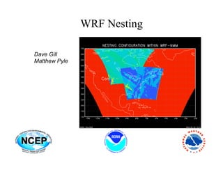
1. WRF Nesting
Dave Gill
Matthew Pyle

2. ARW Nesting

3. Nesting Basics - What is a nest
• A nest is a finer-resolution model run. It may be embedded
simultaneously within a coarser-resolution (parent) model run, or
run independently as a separate model forecast.
• The nest covers a portion of the parent domain, and is driven
along its lateral boundaries by the parent domain.
• Nesting enables running at finer resolution without the following
problems:
• Uniformly high resolution over a large domain - prohibitively
expensive
• High resolution for a very small domain with mismatched time
and spatial lateral boundary conditions

4. Nesting Basics - NMM
• The focus is on static, one- or two-way nesting
• Static: The nest location is fixed in space
• One-way: Information exchange between the parent and the nest is strictly
down-scale. The nest solution does not feedback to the coarser/parent
solution.
• Two-way: Information exchange between the parent and the nest is bi-
directional. The nest feedback impacts the coarse-grid domain’s solution.
• Fine grid input is for non-meteorological variables.

5. Nesting Basics - ARW
• One-way nesting via multiple model forecasts
• One-way nesting with a single model forecast, without feedback
• One-way/two-way nesting with a single input file, all fields
interpolated from the coarse grid
• One-way/two-way nesting with multiple input files, each domain
with a full input data file
• One-way/two-way nesting with the coarse grid data including all
meteorological fields, and the fine-grid domains including only the
static files
• One-way/two-way nesting with a specified move for each nest
• One-way/two-way nesting with a automatic move on the nest
determined through 500 mb low tracking

6. Some Nesting Hints
• Allowable domain specifications
• Defining a starting point
• Illegal domain specifications
• 1-way vs 2-way nesting

7. Two nests on the same “level”, with a common
parent domain
Nest #1 Parent
domain
Nest #2

8. Two levels of nests, with nest #1 acting as the parent
for nest #2
Parent
domain
Nest #1
Nest #2

9. These are all OK
Telescoped to any depth
Any number of siblings
1
4
2
3
5
6
7

10. Some Nesting Hints
• Allowable domain specifications
• Defining a starting point
• Illegal domain specifications
• 1-way vs 2-way nesting

11. ARW Coarse Grid Staggering
i_parent_start
j_parent_start

12. ARW Coarse Grid Staggering 3:1 Ratio
Starting
Location
I = 31
CG … 30 31 32 33 34

13. ARW Coarse Grid Staggering 3:1 Ratio
Feedback:
U : column
V : row
T : cell

14. NMM Coarse/Fine Overlay

15. NMM Telescopic E-Grid
• Interpolations are done on the rotated latitude/longitude projection.
The fine grid is coincident with a portion of the high-resolution grid
that covers the entire coarse grid.
• The nested domain can be placed anywhere within the parent domain
and the nested grid cells will exactly overlap the parent cells at the
coincident cell boundaries.
• Coincident parent/nest grid points eliminate the need for complex,
generalized remapping calculations, and enhances model performance
and portability.
• The grid design was created with moving nests in mind.

16. An odd grid ratio introduces parent/nest points being
coincident, and a 3:1 ratio is preferred as it has been
extensively tested.
H v H v H v H v
v H v H v H v
H v H v H v H
v H v H v H v H
H v H v H v H
nest “dx”
v H v H v H v
H v H v H v H v
parent “dx”

17. Some Nesting Hints
• Allowable domain specifications
• Defining a starting point
• Illegal domain specifications
• 1-way vs 2-way nesting

18. Not OK for 2-way
Child domains may not have overlapping points in the
parent domain (1-way nesting excluded).
1
2
3

19. Not OK either
Domains have one, and only one, parent -
(domain 4 is NOT acceptable even with 1-way nesting)
1
3
2
4

20. Some Nesting Hints
• Allowable domain specifications
• Defining a starting point
• Illegal domain specifications
• 1-way vs 2-way nesting

21. Nesting Performance
• The size of the nested domain may need to be
chosen with computing performance in mind.
• Assuming a 3:1 ratio and the same number of grid
cells in the parent and nest domains, the fine grid
will require 3x as many time steps to keep pace
with the coarse domain.
• A simple nested domain forecast is approximately
4x the cost of just the coarse domain.
• Don’t be cheap on the coarse grid, 2x as many CG
points in only a 25% nested forecast time increase.

22. NMM: Initial Conditions
• Simple horizontal bilinear interpolation of the parent initial conditions
is used to initialize all meteorological fields on the nest.
• A nearest-neighbor approach is adopted for prescribing most of the
land-state variables.
• Topography and land-sea mask are redefined over the nested domain
using the appropriate “nest level” of WPS info from geogrid.
• Quasi-hydrostatic mass balancing is carried out after introducing the
high-resolution topography.

23. ARW: 2-Way Nest with 2 Inputs
Coarse and fine grid domains must WPS
FG
start at the same time, fine domain may WPS
end at any time CG
Feedback may be shut off to produce
a 1-way nest (cell face and cell average) real.exe
CG: multiple times
FG: one time
Any integer ratio for coarse to fine is
permitted, odd is usually chosen for
real-data cases wrf d01
input
wrf d01
bdy
wrf d02
input
Options are available to ingest only the
static fields from the fine grid, with the
coarse grid data horizontally interpolated wrf.exe
to the nest WRF
CG + FG

24. ARW: 2-Way Nest with 2 Inputs
No vertical nesting WPS
FG
WPS
Usually the same physics are run on all CG
of the domains (excepting cumulus)
The grid distance ratio is not strictly tied real.exe
to the time step ratio CG: multiple times
FG: one time
Topography smoothly ramps from coarse
grid to the fine grid along the interface wrf d01
input
wrf d01
bdy
wrf d02
input
along the nest boundary
All fine grids must use the nested lateral
boundary condition wrf.exe
WRF
CG + FG

25. ARW: 2-Way Nest with 1 Input
WPS
CG
ideal CG real CG
Single time multi-times
wrf wrf wrf
input input bdy
wrf CG+FG wrf CG+FG
full fcst full fcst

26. ARW: 2-Way Nest with 1 Input
A single namelist column entry is tied to each WPS
domain CG
The horizontal interpolation method, feedback,
and smoothing are largely controlled through real CG
multi-times
the Registry file
For a 3:1 time step ratio, after the coarse grid
is advanced, the lateral boundaries for the fine wrf wrf
input bdy
grid are computed, the fine grid is advanced
three time steps, then the fine grid is fed back
to the coarse grid (recursively, depth first)
wrf CG+FG
full fcst
Helpful run*.tar files are located in the
./WRFV3/test/em_real directory

27. ndown: 1-Way Nest with 2 Inputs
WPS
Separate WRF forecast runs, separate
WPS
FG real pre-processor runs, intervening
CG
ndown.exe run
real CG
multi-times
real FG
single time
Same restrictions for nest ratios
Can start at any time that an output time
wrf
input
wrf
bdy
wrf
input
from the coarse grid was created
Boundary condition frequency for the
wrf CG
full fcst
fine grid is set to coarse grid output
frequency
wrf
input wrf FG
ndown full fcst
CG fcst +
wrf FG initial wrf
out bdy

28. Some Nesting Hints
• Allowable domain specifications
• Defining a starting point
• Illegal domain specifications
• 1-way vs 2-way nesting
• Nest logic in WRF source code
• Nest information in the Registry

29. Allocate and Initialize a Nest
DO WHILE ( nests_to_open( grid , nestid , kid ) )
a_nest_was_opened = .true.
CALL med_pre_nest_initial ( grid , nestid , &
config_flags )
CALL alloc_and_configure_domain ( &
domain_id = nestid , &
grid = new_nest , &
parent = grid , &
kid = kid )
CALL Setup_Timekeeping (new_nest)
CALL med_nest_initial ( grid , new_nest, &
config_flags )
END DO

30. All Siblings get Processed
DO WHILE ( ASSOCIATED( grid_ptr ) )
CALL set_current_grid_ptr( grid_ptr )
CALL solve_interface ( grid_ptr )
CALL domain_clockadvance ( grid_ptr )
CALL domain_time_test( grid_ptr, &
'domain_clockadvance' )
grid_ptr => grid_ptr%sibling
END DO

31. Recursive Nest Depth
DO kid = 1, max_nests
IF ( ASSOCIATED( grid_ptr%nests(kid)%ptr ) ) THEN
CALL set_current_grid_ptr( grid_ptr%nests(kid)%ptr )
CALL med_nest_force ( grid_ptr , &
grid_ptr%nests(kid)%ptr , config_flags )
grid_ptr%nests(kid)%ptr%start_subtime = &
domain_get_current_time(grid) - &
domain_get_time_step(grid)
grid_ptr%nests(kid)%ptr%stop_subtime = &
domain_get_current_time(grid)
CALL integrate ( grid_ptr%nests(kid)%ptr )
CALL med_nest_feedback ( grid_ptr , &
grid_ptr%nests(kid)%ptr , config_flags )
END IF
END DO

32. Input vs Interpolating
CALL med_interp_domain( parent, nest )
CALL init_domain_constants ( parent, nest )
IF ( nest_config_flags%input_from_file ) THEN
IF ( nest_config_flags%input_from_file ) THEN
CALL med_initialdata_input_ptr( nest , &
nest_config_flags )
ENDIF

33. Feedback and Domain Sync-ing
CALL med_nest_feedback ( parent , nest , &
config_flags )
CALL start_domain ( nest , .TRUE. )
CALL start_domain ( parent , .TRUE. )

34. NMM Nested LBCs
• Nest boundaries generally are treated in the
same way as the standard parent domain
boundaries:
– outermost row is prescribed
– two rows in from boundary is freely
integrating
– in between is a blending zone (average
of outermost and freely integrating
points)
• The one key difference is frequency of
boundary updates: nested boundaries are
updated at every time step of the parent
domain.

35. NMM Mass Balancing for LBCs
• The parent domain geopotential height, temperature, and
moisture are all vertically interpolated (cubic splines) from the
hybrid surfaces onto standard isobaric levels.
• Using horizontally interpolated information of the height field
from the parent domain, and high-resolution topography from the
nest level, mass is adjusted and revised hybrid surfaces are
constructed.
• T and q: 1) horizontally interpolated to the nest domain on
standard pressure levels, 2) vertically interpolated onto the new
hybrid surfaces
• Approach produces an effective way of updating the nest
interface without much distortion or noise

36. ARW Lateral Smoothing

37. Intermediate Domains
The intermediate domain between a parent and a child is the
resolution of the coarse grid over the size of the fine grid. It
allows the model to re-decompose the domain among all of
the processors.

38. Intermediate Domains - Part 1
grid => nested_grid%intermediate_grid
CALL alloc_space_field ( grid, grid%id , 1 , 2 , .TRUE. ,
grid => parent_grid
CALL model_to_grid_config_rec ( grid%id , &
model_config_rec , config_flags )
CALL couple_or_uncouple_em ( grid , config_flags ,.true. &
# include "em_actual_new_args.inc” )
grid => nested_grid
CALL model_to_grid_config_rec ( grid%id , &
model_config_rec , config_flags )
CALL couple_or_uncouple_em ( grid , config_flags ,.true. &
# include "em_actual_new_args.inc” )

39. Intermediate Domains - Part 1
grid => parent_grid
CALL model_to_grid_config_rec ( grid%id ,
model_config_rec , config_flags )
CALL interp_domain_em_part1 ( grid , &
nested_grid%intermediate_grid, nested_grid, &
config_flags &
# include "em_actual_new_args.inc” )

40. Intermediate Domains - Part 2
grid => nested_grid%intermediate_grid
CALL model_to_grid_config_rec ( nested_grid%id , &
model_config_rec , config_flags )
CALL force_domain_em_part2 ( grid, nested_grid, &
config_flags &
# include "em_actual_new_args.inc")
grid => nested_grid
CALL model_to_grid_config_rec ( grid%id , &
model_config_rec , config_flags )
CALL couple_or_uncouple_em ( grid , config_flags ,.false. &
# include "em_actual_new_args.inc" )
grid => parent_grid
CALL model_to_grid_config_rec ( grid%id , &
model_config_rec , config_flags )
CALL couple_or_uncouple_em ( grid , config_flags ,.false. &
# include "em_actual_new_args.inc" )

41. ARW Masked Interpolation

42. ARW Masked Feedback

43. Some Nesting Hints
• Allowable domain specifications
• Defining a starting point
• Illegal domain specifications
• 1-way vs 2-way nesting
• Nest logic in WRF source code
• Nest information in the Registry

44. What are those “usdf” Options
state real u ikjb dyn_em 2 X
i01rhusdf=(bdy_interp:dt)
"U" "x-wind component" "m s-1”
“f” defines what lateral boundary forcing routine (found in
share/interp_fcn.F) is utilized, colon separates the
additional fields that are required (fields must be
previously defined in the Registry)

45. What are those “usdf” Options
state real landmask ij misc 1 -
i012rhd=(interp_fcnm)u=(copy_fcnm)
"LANDMASK" "LAND MASK (1=LAND, 0=WATER)"
“u” and “d” define which feedback (up-scale) and horizontal
interpolation (down-scale) routines (found in
share/interp_fcn.F) are utilized
Default values (i.e. not a subroutine name listed in the
parentheses) assume non-masked fields
At compile-time, users select options

46. What are those “usdf” Options
state real ht ij misc 1 - i012rhdus "HGT"
"Terrain Height" "m"
“s” if the run-time option for smoothing is activated, this field is
to be smoothed - only used for the parent of a nest domain,
smoothing is in the area of the nest, excluding the outer row
and column of the nest coverage
Whether or not smoothing is enabled is a run-time option from
the namelist

47. Special IO Stream #2 Fields
state real msft ij misc 1 -
i012rhdu=(copy_fcnm) "MAPFAC_M"
"Map scale factor on mass grid" "”
state real msfu ij misc 1 X
i012rhdu=(copy_fcnm) "MAPFAC_U"
"Map scale factor on u-grid" "”
state real msfv ij misc 1 Y
i012rhdu=(copy_fcnm) "MAPFAC_V"
"Map scale factor on v-grid" ""