SlideShare a Scribd company logo
1 of 19
Dr.Y.Narasimha MurthyPh.D
yayavaram@yahoo.com
1
RTOS APPLICATIONS
RTOS find applications in various fields of engineering and technology .Some of them include
Control systems, Image processing, Fault Tolerance systems etc.
(i).RTOS for control systems
Many real-time systems are embedded in sensors and actuators and function as digital
controllers. The term plant in the block diagram below refers to a controlled system, for
example, an engine, a brake, an aircraft, a patient. The state of the plant is monitored by sensors
and can be changed by actuators. The real-time (computing) system estimates from the sensor
readings the current state of the plant and computes a control output based on the difference
between the current state and the desired state which is the reference input.
Let us consider an example of PID Controller with single input and single output
Which is common in practice. The analog sensor reading y(t) gives the measured state of the
plant at time t.
Let e(t) = r (t) − y(t) denote the difference between the desired state r (t) and the
measured state y(t) at time t . The output u(t) of the controller consists of three terms: a term that
is proportional to e(t), a term that is proportional to the integral of e(t) and a term that is
proportional to the derivative of e(t).
The entire process can be done by an infinite timed loop
 set timer to interrupt periodically with period T ;
Dr.Y.Narasimha MurthyPh.D
yayavaram@yahoo.com
2
 at each timer interrupt, do
 do analog-to-digital conversion to get y;
 compute control output u;
 output u and do digital-to-analog conversion;
 end do;
Here, we assume that the system provides a timer. Once set by the program, the timer generates
an interrupt every T units of time until its setting is cancelled.
The length T of time between any two consecutive instants at which y(t) and r (t) are sampled is
called the sampling period. T is a key design choice. The behavior of the resultant digital
controller critically depends on this parameter.
Ideally we want the sampled data version to behave like the analog version. This can be done by
making the sampling period small. However, a small sampling period means more frequent
control-law computation and higher processor-time demand. We want a sampling period T that
achieves a good compromise.
In making this selection, two factors are to be considered. The first is the perceived
responsiveness of the overall system (i.e., the plant and the controller). Oftentimes, the system is
operated by a person (e.g., a driver or a pilot). The operator may issue a command at anytime,
say at t . The consequent change in the reference input is read and reacted to by the digital
controller at the next sampling instant. This instant can be as late as t + T . Thus, sampling
introduces a delay in the system response. The operator will feel the system sluggish when the
delay exceeds a tenth of a second. Therefore, the sampling period of any manual input should
be under this limit.
The second factor is the dynamic behavior of the plant. We want to keep the oscillation
in its response small and the system under control. To explain this let us consider a disk drive
controller. The plant in this example is the arm of a disk. The controller is designed to move the
arm to the selected track each time when the reference input changes.
At each change, the reference input r (t) is a step function from the initial position to the
final position .In figures below these positions are represented by 0 and 1, respectively, and
the time origin is the instant when the step in r (t) occurs. The dashed lines in (a) give the output
u(t) of the analog controller and the observed position y(t) of the arm as a function of time. The
Dr.Y.Narasimha MurthyPh.D
yayavaram@yahoo.com
3
solid lines in the lower and upper graphs give, respectively, the analog control signal constructed
from the digital outputs of the controller and the resultant observed position y(t) of the arm. At
the sampling rate shown here, the analog and digital versions are essentially the same.
The solid lines in (b) give the behavior of the digital version when the sampling period is
increased by 2.5 times.
Dr.Y.Narasimha MurthyPh.D
yayavaram@yahoo.com
4
The oscillatory motion of the arm is more pronounced but remains small enough to be
acceptable. However, when the sampling period is increased by five times, as shown in figure
(c), the arm requires larger and larger control to stay in the desired position; when this occurs,
the system is said to have become unstable.
In general, the faster a plant can and must respond to changes in the reference input,
the faster the input to its actuator varies, and the shorter the sampling period should be. We
can measure the responsiveness of the overall system by its rise time R. This term refers to
the amount of time that the plant takes to reach some small neighborhood around the final
state in response to a step change in the reference input.
In the example in the figure above, a small neighborhood of the final state means the values of
y(t) that are within 5 percent of the final value. Hence, the rise time of that system is
approximately equal to 2.5.
Multirate Systems : A plant typically has more than one degree of freedom. Its state is defined
by multiple state variables (e.g., the rotation speed, temperature, etc. of an engine or the tension
and position of a video tape). Therefore, it is monitored by multiple sensors and controlled by
multiple actuators.
One can consider a multivariate (i.e., multi-input/multi-output) controller for such a plant as a
system of single-output controllers. Because different state variables may have different
dynamics, the sampling periods required to achieve smooth responses from the perspective of
different state variables maybe different. [For example, because the rotation speed of a engine
changes faster than its temperature, the required sampling rate for RPM (Rotation Per Minute)
control is higher than that for the temperature control.]
Of course, we can use the highest of all required sampling rates. This choice simplifies the
controller software since all control laws are computed at the same repetition rate. However,
some control-law computations are done more frequently than necessary; some processor time is
wasted. To prevent this waste, multivariate digital controllers usually use multiple rates and are
therefore called multirate systems. Many times, the sampling periods used in a multirate system
are related in a harmonic way, that is, each longer sampling period is an integer multiple of every
shorter period.
This multirate controller controls only flight dynamics. The control system on board an aircraft is
considerably more complex which typically contains many other equally critical subsystems
Dr.Y.Narasimha MurthyPh.D
yayavaram@yahoo.com
5
(e.g., air inlet, fuel, hydraulic, brakes, and anti-ice controllers) and many not so critical
subsystems (e.g., lighting and environment temperature controllers). So, in addition to the flight
control-law computations, the system also computes the control laws of these subsystems.
Controllers in a complex monitor and control system are typically organized hierarchically. One
or more digital controllers at the lowest level directly control the physical plant. Each output of a
higher-level controller is a reference input of one or more lower-level controllers.
For example, a patient care system may consist of microprocessor-based controllers that monitor
and control the patient’s blood pressure, respiration, glucose, and so forth. There may be a
higher-level controller (e.g., an expert system) which interacts with the operator (a nurse or
doctor) and chooses the desired values of these health indicators. While the computation done by
each digital controller is simple and nearly deterministic, the computation of a high level
controller is likely to be far more complex and variable. While the period of a low level control-
law computation ranges from milliseconds to seconds, the periods of high-level control-law
computations may be minutes, even hours.
Figure below shows a more complex example: the hierarchy of flight control, avionics,and air
traffic control systems .
The Air Traffic Control (ATC) system is at the highest level. It regulates the flow of flights to
each destination airport. It does so by assigning to each air craft an arrival time at each metering
(or waypoint) en route to the destination: The aircraft is supposed to arrive at the metering fix at
the assigned arrival time. At any time while in flight, the assigned arrival time to the next
metering fix is a reference input to the on-board flight management system. The flight
management system chooses a time-referenced flight path that brings the aircraft to the next
metering fix at the assigned arrival time. The cruise speed, turn radius, decent/accent rates, and
so forth required to follow the chosen time-referenced flight path are the reference inputs to the
flight controller at the lowest level of the control hierarchy.
As another example for higher levels of control let us consider a control system of robots that
perform assembly tasks in a factory for example. Path and trajectory planners at the second level
determine the trajectory to be followed by each industrial robot. These planners typically take as
an input the plan generated by a task planner, which chooses the sequence of assembly steps to
be performed. In a space robot control system, there may be a scenario planner, which
Dr.Y.Narasimha MurthyPh.D
yayavaram@yahoo.com
6
determines how a repair or rendezvous function should be performed. The plan generated by this
planner is an input of the task planner.
Fig: Air traffic/flight control hierarchy
An Air Traffic Control (ATC) system is an excellent example for Real-Time Command and
Control. The ATC system monitors the aircraft in its coverage area and the environment
(e.g, weather condition) and generates and presents the information needed by the operators
(i.e., the air traffic controllers). Outputs from the ATC system include the assigned arrival
Dr.Y.Narasimha MurthyPh.D
yayavaram@yahoo.com
7
times to metering fixes for individual aircraft. As stated earlier, these outputs are reference
inputs to on-board flight management systems. Thus, the ATC system indirectly controls the
embedded components in low levels of the control hierarchy. In addition, the ATC system
provides voice and telemetry links to on-board avionics. Thus it supports the communication
among the operators at both levels (i.e., the pilots and air traffic controllers).The ATC system
gathers information on the “state” of each aircraft via one or more active radars. Such a radar
interrogates each aircraft periodically. When interrogated, an air- craft responds by sending to
the ATC system its “state variables”: identifier, position, altitude, heading, and so on.
Fig:An architecture of air traffic control system
Dr.Y.Narasimha MurthyPh.D
yayavaram@yahoo.com
8
The ATC system processes messages from aircraft and stores the state information thus obtained
in a database. This information is picked up and processed by display processors. At the same
time, a surveillance system continuously analyzes the scenario and alerts the operators whenever
it detects any potential hazard (e.g., a possible collision). Again, the rates at which human
interfaces (e.g., keyboards and displays) operate must be at least 10 Hz. The other response times
can be considerably larger.
For example, the allowed response time from radar inputs is one to two seconds, and the period
of weather updates is in the order of ten seconds.
From the above example, it is clear that a command and control system bears little resemblance
to low-level controllers. In contrast to a low-level controller whose workload is either purely or
mostly periodic, a command and control system also computes and communicates in response to
sporadic events and operators’ commands. Furthermore, it may process image and speech, query
and update databases, simulate various scenarios, and the like. The resource and processing time
demands of these tasks can be large and varied. Fortunately, most of the timing requirements of a
command and control system are less stringent. Whereas a low-level control system typically
runs on one computer or a few computers connected by a small network or dedicated links, a
command and control system is often a large distributed system containing tens and hundreds of
computers and many different kinds of networks.
In this respect, it resembles interactive, on-line transaction systems (e.g., a stock price quotation
system) which are also sometimes called real-time systems.
(ii). RTOS for image processing:
Real-time image processing (RTIP) promises to be at the heart of many developments in
computer technology: context aware computers, mobile robots, Medical augmented reality and
the subject of research — video-based interfaces for human computer interaction. These
applications have significant demands not only in terms of processing power: they must achieve
real-time, low latency response to their visual input. The modern operating systems provide a
wealth of multimedia features which are usually oriented towards the playback or recording of
media rather than processing in real time.
Dr.Y.Narasimha MurthyPh.D
yayavaram@yahoo.com
9
One can think of three types of Real Time Imaging systems. Soft real time Imaging, Firm Real
Time Imaging and Hard Real Time Imaging systems.
In Soft real-time imaging systems, missed deadlines manifest as performance degradation. For
example , the image processing used in an animated cartoon system. Here each cartoon frame is
separately processed and only played back in real-time at the end. So, while exceptionally slow
processing of each frame might be annoying, it will not affect the end product. Most
entertainment systems tend to fall into the category of soft real-time imaging.
On the other hand, “firm” real-time imaging systems can tolerate a few missed deadlines. In
many imaging systems, for example, a common deadline is that the screen be updated at least 30
times per second. If this deadline is missed frequently, the image will not appear as continuous
motion and the system will have failed. However, a small number of missed deadlines are
acceptable.
But in a “hard” real-time imaging system even one missed deadline can lead to disaster. For
example, consider the need to identify an enemy aircraft using an image- matching algorithm
within a few milliseconds. Failure to meet that deadline, identify the enemy and destroy it can
have catastrophic consequences. This class of real-time imaging systems is the most challenging
to build.
Multimedia systems are complex real-time imaging systems that incorporate powerful
processors, high-speed networks and massive storage devices. Significant research is focused on
developing high bus bandwidth and display capability for the vast number of large images that
must be processed. For example, until very recently, high resolution real-time could only be
obtained using specialized image processing boxes such as Silicon Graphic’s machines. Today,
such images can be processed on modestly-high performance PCs. Another real-time imaging
concern is in the development of compression and decompression techniques that effectively
manage data loss, compression rate, and decompression rate and performance predictability.
Different media representations and handling mechanisms are often necessary for real-time
processing. The operating system itself must also be capable of efficient, low-latency response
and processing.
Mac OS X provides a robust operating system with excellent latency performance and a rich
multimedia framework that can be applied, with some provisions to RTIP applications.
For real time image processing the following provisions are required
Dr.Y.Narasimha MurthyPh.D
yayavaram@yahoo.com
10
• high resolution, high frame rate video input
• low latency video input
• low latency operating system scheduling
• high processing performance.
In the most general terms, image processing attempts to extract information from the outside
world through its visual appearance. Therefore adequate information must be provided to the
processing algorithm by the video input hardware. Precise requirements will, depend on the
algorithm and application but usually both spatial and temporal resolution are important.
Broadcast video provides a practical reference point as most cameras provide images in formats
derived from broadcast standards regardless of their computer interface (analog, USB etc).
Higher resolution in both spatial and temporal sampling is desirable for many applications.
Low latency video input:
All video input systems have intrinsic sources of latency in their hardware and transmission
schemes. Indeed, the relatively sparse temporal sampling (frame rate) typical for video can itself
be thought of as a source of latency equal to the frame duration. Higher frame rates therefore
allow for lower latency and more responsive RTIP systems. Additional latency occurs in the
transmission of video from the camera to the computer interface. The sequential nature of almost
all video frame transmission also imposes latency equal to the frame transmission time (which is
usually close to the frame duration in order to minimise bandwidth requirements). This applies to
digital transmission schemes over USB or Fire wire just as it does to analogue transmission.
Low latency operating system scheduling:
Once the video signal arrives at the computer it will be processed and passed between a
number of software components. These components will depend on the type of video capture
hardware in use, but generally and in the minimum case there will be a driver component and
an application that performs the image processing. The driver is responsible for receiving the
transmission and presenting the video frame as a buffer of pixels and is of course provided by
the operating system vendor or hardware vendor. This pixel buffer is then processed by the
application which would then typically produce some output for the user or provide
information to other application software running on the system.
Dr.Y.Narasimha MurthyPh.D
yayavaram@yahoo.com
11
The ability of the Real Time operating system to respond to incoming video data and to
schedule each of these software components to run as soon as its data are available has a crucial
impact on system latency. If no input data is to be lost, buffering (and hence additional latency)
must be introduced to cover both lag and any variation in when data is available and when it is
passed to the next component. This lag and variation is related to system interrupt latency and
scheduling latency.
For example the Real Time OS Mac OS X has excellent low latency performance even under
heavy system load as evidenced by its reliable behaviour with low latency audio software.
High Processing performance:
Image processing algorithms are very bandwidth and processor speed intensive. High bandwidth
memory architecture, effective caching and high performance processors are necessary for an
RTIP platform. Altivec is an important factor in achieving good performance, as image
processing algorithms are usually highly parallel and therefore well suited to SIMD optimization.
Recent developments in processor hardware architecture [ for ex : in changes in Macintosh
hardware architecture] are also very promising for RTIP, in particular the emphasis on memory
bandwidth.
Video Capture Hardware
Video capture hardware performs the vital role of handling the reception of the video signal
into the computer and presenting to the processor in a suitable form. Some hardware
integrates both camera and digitization functions together, such as the DV video cameras, and
USB Webcams. Other systems perform only digitization of an analog video signal provided
by an external camera. These devices are then connected to a suitable system bus (PCI,
Firewire or sometimes USB).
Suitable devices for RTIP must provide high resolution, high frame rate video at low latency.
Making the video signal available in an uncompressed format to the image processing software
with low CPU overhead is also important. These requirements unfortunately exclude
many common video input devices which provide only low quality input or introduce latency
through their compression or transmission schemes.
USB hardware
Both cameras and digitizers are available which use the common and convenient USB for
Dr.Y.Narasimha MurthyPh.D
yayavaram@yahoo.com
12
communication to the host computer. Unfortunately the low bandwidth of USB 1.1 (11Mbps)
is insufficient to convey high resolution video at high frame rate. Most devices are limited to
320x240 pixels at 30fps(frames per second). Some devices provide higher resolution at lower
frame rates. Other devices achieve acceptable frame rates and resolution but they must employ a
compression scheme such as MPEG to limit their data rate for USB. The MPEG compression
schemes not only degrade the visual quality of the incoming signal but usually add latency to the
video input stream. USB 2.0 offers sufficient bandwidth for high quality video.
PCI hardware
The most traditional hardware for RTIP (Real Time Image Processing) is the combination of an
analogue camera and a PCI based video digitizer. This approach can offer excellent performance
as the video digitizer can perform useful preprocessing and move the video frame buffers via
DMA. This style of hardware must be supported by all versions of RTOS..
The Video recording model tries to avoid dropping frames at all costs by adding buffers to the
video stream and demanding priority scheduling. An RTIP system would usually prioritize
latency over the dropping of frames and therefore introduce as few buffers to the video stream as
possible. Furthermore, if critical time deadlines are not being met (such as processing time for
other parts of the RTIP system or frame drops due to frame handling taking too long) the
behavior of an RTIP scheme will be different to that of a recording scheme.
Even if the RTIP system does not require the display of video as part of its output, it is always
important to be able to monitor and preview the video stream at various stages of processing.
Certain RTOSes like QuickTime includes functions which perform hardware accelerated display
of buffer with some pixel formats and appropriate conversions for buffers of many other pixel
formats.
Real-time imaging design issues: One challenge in designing real-time image processing
systems is the high computational intensity of the algorithms involved. For example, image
filtering each pixel separately for a 1024 by 1024 pixel display can be very costly in terms of
memory requirements and processing time. Typical hardware for real-time imaging applications
involves high-performance computers with firmware support for complex instruction sets and
algorithmic transformations. However, commercial pixel processors, where one processor is
assigned to each pixel, are available and inexpensive. Also, scalable structures, such as the field
programmable gate arrays, are increasingly being used. But building systems with highly
Dr.Y.Narasimha MurthyPh.D
yayavaram@yahoo.com
13
specialized processors is not very easy because there is usually limited expertise with these
specialized environments. Also, tool support is generally thin because of overall low market
demand.
Whatever the hardware platform, many use an object-oriented software approach because of the
high-level language support it provides. Such approaches can incur significant performance
penalties in terms of memory utilization and time. They can also introduce behavior uncertainty
because of garbage collection. For example, in an object-oriented language if every pixel were
treated as an object images of faces; analysis of medical images and fingerprints; robotics and
artificial intelligence systems.
•Multimedia/virtual reality including geometric representations of objects and surfaces; models
of scene illumination; geometric representations of image parts; spatial arrangements and image
representation; 3D object description; specialized computation techniques.
• Algorithms comprising any algorithms for image processing not covered in other areas; multi-
image processing; image segmentation.
• Software engineering constituting tools, languages and engineering methodologies unique to
real-time imaging; imaging aesthetics; cognitive perception and paradigms.
(iii). Embedded RTOS for voice over IP(voIP)
Voice over IP (VOIP) uses the Internet Protocol (IP) to transmit voice as packets over an IP
network. So VOIP can be achieved on any data network that uses IP, like Internet, Intranets and
Local Area Networks (LAN). Here the voice signal is digitized, compressed and converted to IP
packets and then transmitted over the IP network. It is an advancing technology that is used to
transmit voice over the internet or a local area network using internet protocol (IP).This
technology provides enhanced features such as low cost compared to the traditional Public
Switched Telephone Network (PSTN). VoIP system costs as much as half the traditional PSTN
system in the field of voice transmission. This is because of the efficient use of bandwidth
requiring fewer long-distance trunks between switches.
The voice over internet protocol system is found to be the successful alternative to the traditional
PSTN communication system due to its advanced features. The voice signal is processed through
Dr.Y.Narasimha MurthyPh.D
yayavaram@yahoo.com
14
the internet based network during the communication. The conceptual diagram of VoIP system is
shown in Fig.below.
The basic steps in derivation of the designed VoIP system are:
 The original speech signal is fed in to the system and the speech samples are taken from .
 The speech signal is then encoded with G.711a and Speex speech encoders, which is the
compressed version of the input signal. G.711a is the standard used for the
communication purpose and is a high bit rate Pulse Code Modulation codec. It works at
sampling rate of 8 kHz and uses and compresses the 16 bit audio samples into 8bits . The
Code Excited Linear Prediction (CELP) Speex codec is an open source codec developed
for the packet network and VoIP applications.The Speex supports three different
sampling rates narrowband (8 kHz), wideband (16 kHz) and ultra-wideband (32 kHz).
 The compressed signal is then packetized into VoIP packets to transfer it to the IP
network.
 The speech signal is degraded due to the various network impairments including delay,
jitter and packet loss during VoIP communications. The network impairments are
introduced through the lab WANem emulator .
 The degraded VoIP signal is depacketized and then decoded with G.711a and Speex
decoders.
 The performance is evaluated with Perceptual Evaluation of Speech Quality (PESQ)
measurement defined by ITU-T recommendation P.862 . After comparing the degraded
Dr.Y.Narasimha MurthyPh.D
yayavaram@yahoo.com
15
signal with the original one, the PESQ measurement gives the subjective measurement as
Mean Opinion Scores (MOS) value from -0.5 to 4.5.
 The VoIP signal is processed through various signal processing algorithms to evaluate the
performance of the system.
Voice quality in communication systems is influenced by many factors such as packet delay,
jitter, packet loss and type & amount of voice compression. Due to these distortion factors, the
speech signal is not of very good quality over the VoIP network. Delay is the time taken by the
voice to reach from talker’s mouth to the listener’s ear. Round trip delay is the sum of two one-
way delays that occur in the user’s call. In VoIP system, the propagation delay is also affected by
two additional delays such as packeting delay and the time required for propagating the packet
through the network. This varies the propagation delay during the transmission.
The variation in the arrival time of the packets at the receiver end leads to jitter, which affects the
perceived quality of conversation very badly. The sender is expected to transmit each voice
packet at a regular interval. But jitter affects the speech in such a way that all voice packets do
not arrive at the right time at the decoder and thus reconstructed speech would not be continuous,
at the receiver end. The transmission time of a packet through IP network varies due to queuing
effect in the interconnected network. The packet loss is the percentage of the lost packets during
the transportation due to various network conditions such as buffer overflow, network congestion
etc. The delay and jitter also contribute to the packet losses and these results in harmful effects
on the quality of VoIP signal. Due to the real time requirement for interactive speech
transmission, it is usually impossible for the receivers to request the sender to retransmit the lost
packets. When voice packets do not arrive before their payout time, they are considered as lost
and cannot be played when they are received. Even a single lost packet may generate audible
distortion in the decoded speech signal.
To analyze the effect of packet loss on the quality of the degraded VoIP output, the spectral
analysis was performed in time and frequency by using various signal processing algorithms.
The real-time establishment scheme assumes that scheduling in the hosts and in the nodes will be
deadline-based. Each real-time packet in the node is given a deadline, which is the time by which
it is to be serviced. Let di, n be the local delay bound assigned to channel i in node n. A packet
Dr.Y.Narasimha MurthyPh.D
yayavaram@yahoo.com
16
traveling on that channel and arriving at that node at time to will usually be assigned a node
deadline equal to to+di, n .
The scheduler maintains at least two queues : one for real-time packets and the other for all other
types of packets and all local tasks. The first queue has higher priority, is ordered according to
packet deadlines, and served in order of increasing deadlines. The second queue can be replaced
by multiple queues, managed by a variety of policies.
At channel establishment time, each intermediate node checks whether it will be able to accept
packets at the rate declared by the sender. However, malicious users or faulty behavior by system
components could cause packets to arrive into the network at a much higher rate than the
declared maximum value, 1/x min. This can prevent the satisfaction of the delay bounds
guaranteed to other clients of the real-time service. A solution to this problem consists of
providing distributed rate control by extending the deadlines of the ‘‘offending’’ packets. The
deadline assigned to an offending packet would equal the deadline that packet would have if it
had obeyed the xmin constraints declared at connection establishment time.
(iv).RTOS for fault tolerant applications :
Fault tolerance is the ability to continue operating despite the failure of a limited subset of their
hardware or software. So the goal of the system designer is to ensure that the probability of
system failure is acceptably small. There can be either hardware fault or software fault, which
disturbs the real time systems to meet their deadlines.
Real time systems are systems in which there is a guaranty for timely response by the computer
to external input. Real time applications have to function correctly even in presence of faults.
Fault tolerance can be achieved by either hardware or software or time redundancy. Safety-
critical applications have strict time and cost constraints, which means that not only faults have
to be tolerated but also the constraints should be satisfied. Deadline scheduling means that the
task with the earliest required response time is processed. The most common scheduling
algorithms are : Rate Monotonic(RM) and Earliest deadline first(EDF).
In soft real-time systems it is more important to economically detect a fault as soon as possible
rather than to mask a fault. Examples of soft real-time systems are all kind of airline reservation,
banking, and E-commerce applications.
Dr.Y.Narasimha MurthyPh.D
yayavaram@yahoo.com
17
There are three types of faults: Permanent, intermittent, and transient. A permanent fault does not
die away with time, but remains until it is repaired as the affected unit is replaced. This is an
intermittent fault cycle between the fault–active and fault benign states. A transient fault dies
away after some time. Fault detection can be done either online or offline. Online detection goes
on in parallel with normal system operation. Offline detection consists of running diagnostic
tests.
In order to achieve fault tolerance, the first requirement is that transient faults have to be
detected. Several error-detection techniques are there against transient faults: watchdogs,
duplication and few others.
 Watchdogs: In the case of watchdogs program flow or transmitted data is periodically
checked for the presence of errors. In the simplest watchdog scheme, watchdog timer,
monitors the execution time of processes, whether it exceeds a certain limit.
 Duplication: Duplication is an approach to have multiple processors, which are supposed
to put out the same result and compare the results. A discrepancy indicates the existence
Dr.Y.Narasimha MurthyPh.D
yayavaram@yahoo.com
18
of a fault . There are several other error-detections techniques, e.g. signatures, assertions
or the widely-used parity bit check.
 Redundancy : Fault tolerance system is to be kept running despite the failure of some of
its parts, it must have spare capacity to begin. There are two ways to make a system more
resistant to faults. Hardware: this technique relies on adding extra redundant hardware to
a system to make it fault tolerant. -Software: this technique relies on duplicating the
code, process, or even messages, depending on the context. A typical example of where
the above techniques are applied would be the autopilot system on-board a large-sized
passenger aircraft. A passenger aircraft typically consists of a central autopilot system
with two other backups. This is an example of making a system with two other backups.
This is an example of making a system fault tolerant by adding redundant hardware. The
two extra systems will not be used unless the main system is completely broken.
However, this is not sufficient, since in the event that the main system starts behaving
erratically the lives of many people is in danger. The system is therefore also made
resistant to faults using software
However, such measures are only applied for highly critical systems. In general, hardware
redundancy is avoided as far as possible, due to limited resources that are available. Weight of
the system, power consumption, and price constraints make it difficult to employ high hardware
redundancy to make the system fault tolerant. Software redundancy is therefore, more commonly
used to increase fault tolerance of systems. There are few factors that affect the diversity of the
multiple versions. The first factor is the requirements specification. A mistake in the
specification causes a wrong output to be delivered. A second approach is the programming
language. The nature of the language affects the programming style greatly. A third factor is the
numerical algorithms that are used.
Algorithms implemented to a finite precision can behave quite differently for certain sets of
inputs than do theoretical algorithms, which assume infinite precision. A fourth factor is the
nature of the tools that are being used; the probability of common-mode failure might increase. A
fifth factor is the training and quality of the programmers and the management structure. The
major difficulty in software is labor-intensive.
Fault Tolerance Techniques
Dr.Y.Narasimha MurthyPh.D
yayavaram@yahoo.com
19
(i)TMR (Triple Modular Redundancy): Multiple copies are executed and error checking is
achieved by comparing results after completion. In this scheme, the overhead is always on the
order of the number of copies running simultaneously.
(ii) PB (Primary/Backup): The tasks are assumed to be periodic and two instances of each task
(a primary and a backup) are scheduled on a uni-processor system. One of the restrictions of this
approach is that the period of any task should be a multiple of the period of its preceding tasks. It
also assumes that the execution time of the backup is shorter than that of the primary.
(iii) PE (Primary/Exception): It is the same as PB method except that exception handlers are
executed instead of backup programs.
(iv)Primary Backup Fault Tolerance : This is the traditional fault-tolerant approach wherein
both time as well as space exclusions are used. The main idea behind this algorithm is that (a) the
backup of a task need not execute if its primary executes successfully, (b) the time exclusion in
this algorithm ensures that no resource conflicts occur between the two versions of any task,
which might improve the schedulability. Disadvantages in this system are that (a) there is no de-
allocation of the backup copy, (b) the algorithm assumes that the tasks are periodic (the times of
the tasks are predetermined), (c) compatible (the period of one process is an integral multiple of
the period of the other process) and execution time of the backup is shorter than that of the
primary process.
It can be concluded that appropriate use of redundancy is important in Fault Tolerance ,since
too much redundancy increases reliability but potentially decreases the schedulability. Too little
redundancy decreases reliability but increases schedulability. Also, designing, managing
redundancy incurs additional cost, time, and memory and power consumption.
Acknowledgement: Thanks are due to Prof.Philip A.Laplante, Prof.Daniel HeckenBerg,
Dr.T.R.Gopalkrishnan Nair and Prof.A.Christy Persya without whose papers, the preparation of
this material can’t be thought of.

More Related Content

What's hot

Time response and analysis kaushal shah
Time response and analysis kaushal shahTime response and analysis kaushal shah
Time response and analysis kaushal shahKaushal Shah
 
Time Response Analysis
Time Response AnalysisTime Response Analysis
Time Response AnalysisManthan Kanani
 
Chapter 4 Embedded System: Application and Domain Specific
Chapter 4 Embedded System: Application and Domain SpecificChapter 4 Embedded System: Application and Domain Specific
Chapter 4 Embedded System: Application and Domain SpecificMoe Moe Myint
 
INTERRUPT ROUTINES IN RTOS EN VIRONMENT HANDELING OF INTERRUPT SOURCE CALLS
INTERRUPT ROUTINES IN RTOS EN VIRONMENT HANDELING OF INTERRUPT SOURCE CALLSINTERRUPT ROUTINES IN RTOS EN VIRONMENT HANDELING OF INTERRUPT SOURCE CALLS
INTERRUPT ROUTINES IN RTOS EN VIRONMENT HANDELING OF INTERRUPT SOURCE CALLSJOLLUSUDARSHANREDDY
 
SCADA a complete overview
SCADA a complete overviewSCADA a complete overview
SCADA a complete overviewSheikh Ismail
 
Modern Control - Lec 02 - Mathematical Modeling of Systems
Modern Control - Lec 02 - Mathematical Modeling of SystemsModern Control - Lec 02 - Mathematical Modeling of Systems
Modern Control - Lec 02 - Mathematical Modeling of SystemsAmr E. Mohamed
 
Dcs lec01 - introduction to discrete-time control systems
Dcs   lec01 - introduction to discrete-time control systemsDcs   lec01 - introduction to discrete-time control systems
Dcs lec01 - introduction to discrete-time control systemsAmr E. Mohamed
 
UNIT-I-RTOS and Concepts
UNIT-I-RTOS and ConceptsUNIT-I-RTOS and Concepts
UNIT-I-RTOS and ConceptsDr.YNM
 
State space analysis.pptx
State space analysis.pptxState space analysis.pptx
State space analysis.pptxRaviMuthamala1
 
IoT Enabling Technologies
IoT Enabling TechnologiesIoT Enabling Technologies
IoT Enabling TechnologiesPrakash Honnur
 
Lecture 12 time_domain_analysis_of_control_systems
Lecture 12 time_domain_analysis_of_control_systemsLecture 12 time_domain_analysis_of_control_systems
Lecture 12 time_domain_analysis_of_control_systemsSaifullah Memon
 
Structures for discrete time systems
Structures for discrete time systemsStructures for discrete time systems
Structures for discrete time systemsveda C
 
DSP_2018_FOEHU - Lec 03 - Discrete-Time Signals and Systems
DSP_2018_FOEHU - Lec 03 - Discrete-Time Signals and SystemsDSP_2018_FOEHU - Lec 03 - Discrete-Time Signals and Systems
DSP_2018_FOEHU - Lec 03 - Discrete-Time Signals and SystemsAmr E. Mohamed
 
Week 17 digital control sytem
Week 17 digital control sytemWeek 17 digital control sytem
Week 17 digital control sytemCharlton Inao
 
Dcs lec02 - z-transform
Dcs   lec02 - z-transformDcs   lec02 - z-transform
Dcs lec02 - z-transformAmr E. Mohamed
 
state space representation,State Space Model Controllability and Observabilit...
state space representation,State Space Model Controllability and Observabilit...state space representation,State Space Model Controllability and Observabilit...
state space representation,State Space Model Controllability and Observabilit...Waqas Afzal
 
Discrete Fourier Transform
Discrete Fourier TransformDiscrete Fourier Transform
Discrete Fourier TransformAbhishek Choksi
 

What's hot (20)

Time response and analysis kaushal shah
Time response and analysis kaushal shahTime response and analysis kaushal shah
Time response and analysis kaushal shah
 
Time Response Analysis
Time Response AnalysisTime Response Analysis
Time Response Analysis
 
Lecture 5: The Convolution Sum
Lecture 5: The Convolution SumLecture 5: The Convolution Sum
Lecture 5: The Convolution Sum
 
Chapter 4 Embedded System: Application and Domain Specific
Chapter 4 Embedded System: Application and Domain SpecificChapter 4 Embedded System: Application and Domain Specific
Chapter 4 Embedded System: Application and Domain Specific
 
INTERRUPT ROUTINES IN RTOS EN VIRONMENT HANDELING OF INTERRUPT SOURCE CALLS
INTERRUPT ROUTINES IN RTOS EN VIRONMENT HANDELING OF INTERRUPT SOURCE CALLSINTERRUPT ROUTINES IN RTOS EN VIRONMENT HANDELING OF INTERRUPT SOURCE CALLS
INTERRUPT ROUTINES IN RTOS EN VIRONMENT HANDELING OF INTERRUPT SOURCE CALLS
 
SCADA a complete overview
SCADA a complete overviewSCADA a complete overview
SCADA a complete overview
 
Modern Control - Lec 02 - Mathematical Modeling of Systems
Modern Control - Lec 02 - Mathematical Modeling of SystemsModern Control - Lec 02 - Mathematical Modeling of Systems
Modern Control - Lec 02 - Mathematical Modeling of Systems
 
Dcs lec01 - introduction to discrete-time control systems
Dcs   lec01 - introduction to discrete-time control systemsDcs   lec01 - introduction to discrete-time control systems
Dcs lec01 - introduction to discrete-time control systems
 
UNIT-I-RTOS and Concepts
UNIT-I-RTOS and ConceptsUNIT-I-RTOS and Concepts
UNIT-I-RTOS and Concepts
 
State space analysis.pptx
State space analysis.pptxState space analysis.pptx
State space analysis.pptx
 
IoT Enabling Technologies
IoT Enabling TechnologiesIoT Enabling Technologies
IoT Enabling Technologies
 
Lecture 12 time_domain_analysis_of_control_systems
Lecture 12 time_domain_analysis_of_control_systemsLecture 12 time_domain_analysis_of_control_systems
Lecture 12 time_domain_analysis_of_control_systems
 
Bode plot
Bode plotBode plot
Bode plot
 
Lecture 23 24-time_response
Lecture 23 24-time_responseLecture 23 24-time_response
Lecture 23 24-time_response
 
Structures for discrete time systems
Structures for discrete time systemsStructures for discrete time systems
Structures for discrete time systems
 
DSP_2018_FOEHU - Lec 03 - Discrete-Time Signals and Systems
DSP_2018_FOEHU - Lec 03 - Discrete-Time Signals and SystemsDSP_2018_FOEHU - Lec 03 - Discrete-Time Signals and Systems
DSP_2018_FOEHU - Lec 03 - Discrete-Time Signals and Systems
 
Week 17 digital control sytem
Week 17 digital control sytemWeek 17 digital control sytem
Week 17 digital control sytem
 
Dcs lec02 - z-transform
Dcs   lec02 - z-transformDcs   lec02 - z-transform
Dcs lec02 - z-transform
 
state space representation,State Space Model Controllability and Observabilit...
state space representation,State Space Model Controllability and Observabilit...state space representation,State Space Model Controllability and Observabilit...
state space representation,State Space Model Controllability and Observabilit...
 
Discrete Fourier Transform
Discrete Fourier TransformDiscrete Fourier Transform
Discrete Fourier Transform
 

Viewers also liked

Vlsi physical design-notes
Vlsi physical design-notesVlsi physical design-notes
Vlsi physical design-notesDr.YNM
 
UNIT-IV .FINITE STATE MACHINES
UNIT-IV .FINITE STATE MACHINESUNIT-IV .FINITE STATE MACHINES
UNIT-IV .FINITE STATE MACHINESDr.YNM
 
UNIT-V-FPGA &CPLD ARCHITECTURES AND APPLICATIONS
UNIT-V-FPGA &CPLD ARCHITECTURES AND APPLICATIONSUNIT-V-FPGA &CPLD ARCHITECTURES AND APPLICATIONS
UNIT-V-FPGA &CPLD ARCHITECTURES AND APPLICATIONSDr.YNM
 
UNIT-II -DIGITAL SYSTEM DESIGN
UNIT-II -DIGITAL SYSTEM DESIGNUNIT-II -DIGITAL SYSTEM DESIGN
UNIT-II -DIGITAL SYSTEM DESIGNDr.YNM
 
UNIT-II : SEQUENTIAL CIRCUIT DESIGN
UNIT-II  : SEQUENTIAL CIRCUIT DESIGN UNIT-II  : SEQUENTIAL CIRCUIT DESIGN
UNIT-II : SEQUENTIAL CIRCUIT DESIGN Dr.YNM
 
UNIT-III-DIGITAL SYSTEM DESIGN
UNIT-III-DIGITAL SYSTEM DESIGNUNIT-III-DIGITAL SYSTEM DESIGN
UNIT-III-DIGITAL SYSTEM DESIGNDr.YNM
 
Arm processors' architecture
Arm processors'   architectureArm processors'   architecture
Arm processors' architectureDr.YNM
 
UNIT-I DIGITAL SYSTEM DESIGN
UNIT-I DIGITAL SYSTEM DESIGN UNIT-I DIGITAL SYSTEM DESIGN
UNIT-I DIGITAL SYSTEM DESIGN Dr.YNM
 
UNIT II-Programming in Linux
UNIT II-Programming in LinuxUNIT II-Programming in Linux
UNIT II-Programming in LinuxDr.YNM
 
UNIT I- CPLD & FPGA ARCHITECTURE & APPLICATIONS
UNIT I- CPLD & FPGA ARCHITECTURE & APPLICATIONSUNIT I- CPLD & FPGA ARCHITECTURE & APPLICATIONS
UNIT I- CPLD & FPGA ARCHITECTURE & APPLICATIONSDr.YNM
 
faults in digital systems
faults in digital systemsfaults in digital systems
faults in digital systemsdennis gookyi
 
Verilog hdl design examples
Verilog hdl design examplesVerilog hdl design examples
Verilog hdl design examplesdennis gookyi
 
PLA Minimization -Testing
PLA Minimization -TestingPLA Minimization -Testing
PLA Minimization -TestingDr.YNM
 
Semi Custom Integrated Circuit Design
 Semi Custom Integrated Circuit Design Semi Custom Integrated Circuit Design
Semi Custom Integrated Circuit DesignDr.YNM
 
UNIT-II CPLD & FPGA Architectures and Applications
UNIT-II CPLD & FPGA  Architectures   and ApplicationsUNIT-II CPLD & FPGA  Architectures   and Applications
UNIT-II CPLD & FPGA Architectures and ApplicationsDr.YNM
 
Vlsi design notes(1st unit) according to vtu syllabus.(BE)
Vlsi  design notes(1st unit) according to vtu syllabus.(BE)Vlsi  design notes(1st unit) according to vtu syllabus.(BE)
Vlsi design notes(1st unit) according to vtu syllabus.(BE)instrumentation_vtu
 
Introduction to image processing-Class Notes
Introduction to image processing-Class NotesIntroduction to image processing-Class Notes
Introduction to image processing-Class NotesDr.YNM
 
Introduction to VLSI Technology
Introduction to VLSI TechnologyIntroduction to VLSI Technology
Introduction to VLSI TechnologyDr.YNM
 
UNIT-III CASE STUDIES -FPGA & CPGA ARCHITECTURES APPLICATIONS
UNIT-III CASE STUDIES -FPGA & CPGA ARCHITECTURES APPLICATIONSUNIT-III CASE STUDIES -FPGA & CPGA ARCHITECTURES APPLICATIONS
UNIT-III CASE STUDIES -FPGA & CPGA ARCHITECTURES APPLICATIONSDr.YNM
 

Viewers also liked (20)

Vlsi physical design-notes
Vlsi physical design-notesVlsi physical design-notes
Vlsi physical design-notes
 
UNIT-IV .FINITE STATE MACHINES
UNIT-IV .FINITE STATE MACHINESUNIT-IV .FINITE STATE MACHINES
UNIT-IV .FINITE STATE MACHINES
 
UNIT-V-FPGA &CPLD ARCHITECTURES AND APPLICATIONS
UNIT-V-FPGA &CPLD ARCHITECTURES AND APPLICATIONSUNIT-V-FPGA &CPLD ARCHITECTURES AND APPLICATIONS
UNIT-V-FPGA &CPLD ARCHITECTURES AND APPLICATIONS
 
UNIT-II -DIGITAL SYSTEM DESIGN
UNIT-II -DIGITAL SYSTEM DESIGNUNIT-II -DIGITAL SYSTEM DESIGN
UNIT-II -DIGITAL SYSTEM DESIGN
 
UNIT-II : SEQUENTIAL CIRCUIT DESIGN
UNIT-II  : SEQUENTIAL CIRCUIT DESIGN UNIT-II  : SEQUENTIAL CIRCUIT DESIGN
UNIT-II : SEQUENTIAL CIRCUIT DESIGN
 
UNIT-III-DIGITAL SYSTEM DESIGN
UNIT-III-DIGITAL SYSTEM DESIGNUNIT-III-DIGITAL SYSTEM DESIGN
UNIT-III-DIGITAL SYSTEM DESIGN
 
Arm processors' architecture
Arm processors'   architectureArm processors'   architecture
Arm processors' architecture
 
UNIT-I DIGITAL SYSTEM DESIGN
UNIT-I DIGITAL SYSTEM DESIGN UNIT-I DIGITAL SYSTEM DESIGN
UNIT-I DIGITAL SYSTEM DESIGN
 
UNIT II-Programming in Linux
UNIT II-Programming in LinuxUNIT II-Programming in Linux
UNIT II-Programming in Linux
 
UNIT I- CPLD & FPGA ARCHITECTURE & APPLICATIONS
UNIT I- CPLD & FPGA ARCHITECTURE & APPLICATIONSUNIT I- CPLD & FPGA ARCHITECTURE & APPLICATIONS
UNIT I- CPLD & FPGA ARCHITECTURE & APPLICATIONS
 
faults in digital systems
faults in digital systemsfaults in digital systems
faults in digital systems
 
test generation
test generationtest generation
test generation
 
Verilog hdl design examples
Verilog hdl design examplesVerilog hdl design examples
Verilog hdl design examples
 
PLA Minimization -Testing
PLA Minimization -TestingPLA Minimization -Testing
PLA Minimization -Testing
 
Semi Custom Integrated Circuit Design
 Semi Custom Integrated Circuit Design Semi Custom Integrated Circuit Design
Semi Custom Integrated Circuit Design
 
UNIT-II CPLD & FPGA Architectures and Applications
UNIT-II CPLD & FPGA  Architectures   and ApplicationsUNIT-II CPLD & FPGA  Architectures   and Applications
UNIT-II CPLD & FPGA Architectures and Applications
 
Vlsi design notes(1st unit) according to vtu syllabus.(BE)
Vlsi  design notes(1st unit) according to vtu syllabus.(BE)Vlsi  design notes(1st unit) according to vtu syllabus.(BE)
Vlsi design notes(1st unit) according to vtu syllabus.(BE)
 
Introduction to image processing-Class Notes
Introduction to image processing-Class NotesIntroduction to image processing-Class Notes
Introduction to image processing-Class Notes
 
Introduction to VLSI Technology
Introduction to VLSI TechnologyIntroduction to VLSI Technology
Introduction to VLSI Technology
 
UNIT-III CASE STUDIES -FPGA & CPGA ARCHITECTURES APPLICATIONS
UNIT-III CASE STUDIES -FPGA & CPGA ARCHITECTURES APPLICATIONSUNIT-III CASE STUDIES -FPGA & CPGA ARCHITECTURES APPLICATIONS
UNIT-III CASE STUDIES -FPGA & CPGA ARCHITECTURES APPLICATIONS
 

Similar to RTOS APPLICATIONS

RTS Short Topics
RTS Short TopicsRTS Short Topics
RTS Short TopicsSilas Kanth
 
Pe 3032 wk 1 introduction to control system march 04e
Pe 3032 wk 1 introduction to control system  march 04ePe 3032 wk 1 introduction to control system  march 04e
Pe 3032 wk 1 introduction to control system march 04eCharlton Inao
 
5107368.ppt
5107368.ppt5107368.ppt
5107368.pptyibe5
 
Control systems and Robotics
Control systems and RoboticsControl systems and Robotics
Control systems and RoboticsJamshedul Islam
 
KNL3353_Control_System_Engineering_Lectu.ppt
KNL3353_Control_System_Engineering_Lectu.pptKNL3353_Control_System_Engineering_Lectu.ppt
KNL3353_Control_System_Engineering_Lectu.pptSherAli984263
 
Discretizing of linear systems with time-delay Using method of Euler’s and Tu...
Discretizing of linear systems with time-delay Using method of Euler’s and Tu...Discretizing of linear systems with time-delay Using method of Euler’s and Tu...
Discretizing of linear systems with time-delay Using method of Euler’s and Tu...IJERA Editor
 
23 richard a. hall - 5287265 - interfacing methods for use in inputting ope...
23   richard a. hall - 5287265 - interfacing methods for use in inputting ope...23   richard a. hall - 5287265 - interfacing methods for use in inputting ope...
23 richard a. hall - 5287265 - interfacing methods for use in inputting ope...Mello_Patent_Registry
 
Some important tips for control systems
Some important tips for control systemsSome important tips for control systems
Some important tips for control systemsmanish katara
 
Design and Control of a Hydraulic Servo System and Simulation Analysis
Design and Control of a Hydraulic Servo System and Simulation AnalysisDesign and Control of a Hydraulic Servo System and Simulation Analysis
Design and Control of a Hydraulic Servo System and Simulation AnalysisIJMREMJournal
 
K10655(hariom) control theory
K10655(hariom) control theoryK10655(hariom) control theory
K10655(hariom) control theorycpume
 

Similar to RTOS APPLICATIONS (20)

Real Time System
Real Time SystemReal Time System
Real Time System
 
RTS Short Topics
RTS Short TopicsRTS Short Topics
RTS Short Topics
 
Pe 3032 wk 1 introduction to control system march 04e
Pe 3032 wk 1 introduction to control system  march 04ePe 3032 wk 1 introduction to control system  march 04e
Pe 3032 wk 1 introduction to control system march 04e
 
C045051318
C045051318C045051318
C045051318
 
5107368.ppt
5107368.ppt5107368.ppt
5107368.ppt
 
Control systems and Robotics
Control systems and RoboticsControl systems and Robotics
Control systems and Robotics
 
Control system unit(1)
Control system unit(1)Control system unit(1)
Control system unit(1)
 
Pid controller
Pid controllerPid controller
Pid controller
 
chap-1(1).pdf
chap-1(1).pdfchap-1(1).pdf
chap-1(1).pdf
 
Chapter 1
Chapter 1Chapter 1
Chapter 1
 
KNL3353_Control_System_Engineering_Lectu.ppt
KNL3353_Control_System_Engineering_Lectu.pptKNL3353_Control_System_Engineering_Lectu.ppt
KNL3353_Control_System_Engineering_Lectu.ppt
 
Discretizing of linear systems with time-delay Using method of Euler’s and Tu...
Discretizing of linear systems with time-delay Using method of Euler’s and Tu...Discretizing of linear systems with time-delay Using method of Euler’s and Tu...
Discretizing of linear systems with time-delay Using method of Euler’s and Tu...
 
23 richard a. hall - 5287265 - interfacing methods for use in inputting ope...
23   richard a. hall - 5287265 - interfacing methods for use in inputting ope...23   richard a. hall - 5287265 - interfacing methods for use in inputting ope...
23 richard a. hall - 5287265 - interfacing methods for use in inputting ope...
 
Ece4510 notes01
Ece4510 notes01Ece4510 notes01
Ece4510 notes01
 
Measurement
MeasurementMeasurement
Measurement
 
M1 Mechatronics.pptx
M1 Mechatronics.pptxM1 Mechatronics.pptx
M1 Mechatronics.pptx
 
AJMS_481_23.pdf
AJMS_481_23.pdfAJMS_481_23.pdf
AJMS_481_23.pdf
 
Some important tips for control systems
Some important tips for control systemsSome important tips for control systems
Some important tips for control systems
 
Design and Control of a Hydraulic Servo System and Simulation Analysis
Design and Control of a Hydraulic Servo System and Simulation AnalysisDesign and Control of a Hydraulic Servo System and Simulation Analysis
Design and Control of a Hydraulic Servo System and Simulation Analysis
 
K10655(hariom) control theory
K10655(hariom) control theoryK10655(hariom) control theory
K10655(hariom) control theory
 

More from Dr.YNM

Introduction to DSP.ppt
Introduction to DSP.pptIntroduction to DSP.ppt
Introduction to DSP.pptDr.YNM
 
Atmel.ppt
Atmel.pptAtmel.ppt
Atmel.pptDr.YNM
 
PIC Microcontrollers.ppt
PIC Microcontrollers.pptPIC Microcontrollers.ppt
PIC Microcontrollers.pptDr.YNM
 
Crystalstructure-.ppt
Crystalstructure-.pptCrystalstructure-.ppt
Crystalstructure-.pptDr.YNM
 
Basics of OS & RTOS.ppt
Basics of OS & RTOS.pptBasics of OS & RTOS.ppt
Basics of OS & RTOS.pptDr.YNM
 
Introducion to MSP430 Microcontroller.pptx
Introducion to MSP430 Microcontroller.pptxIntroducion to MSP430 Microcontroller.pptx
Introducion to MSP430 Microcontroller.pptxDr.YNM
 
Microcontroller-8051.ppt
Microcontroller-8051.pptMicrocontroller-8051.ppt
Microcontroller-8051.pptDr.YNM
 
Introduction to ASICs.pptx
Introduction to ASICs.pptxIntroduction to ASICs.pptx
Introduction to ASICs.pptxDr.YNM
 
VHDL-PRESENTATION.ppt
VHDL-PRESENTATION.pptVHDL-PRESENTATION.ppt
VHDL-PRESENTATION.pptDr.YNM
 
Basics of data communications.pptx
Basics of data communications.pptxBasics of data communications.pptx
Basics of data communications.pptxDr.YNM
 
CPLD & FPGA Architectures and applictionsplications.pptx
CPLD & FPGA Architectures and applictionsplications.pptxCPLD & FPGA Architectures and applictionsplications.pptx
CPLD & FPGA Architectures and applictionsplications.pptxDr.YNM
 
Transient response of RC , RL circuits with step input
Transient response of RC , RL circuits  with step inputTransient response of RC , RL circuits  with step input
Transient response of RC , RL circuits with step inputDr.YNM
 
CISC & RISC ARCHITECTURES
CISC & RISC ARCHITECTURESCISC & RISC ARCHITECTURES
CISC & RISC ARCHITECTURESDr.YNM
 
Lect 4 ARM PROCESSOR ARCHITECTURE
Lect 4 ARM PROCESSOR ARCHITECTURELect 4 ARM PROCESSOR ARCHITECTURE
Lect 4 ARM PROCESSOR ARCHITECTUREDr.YNM
 
Lect 3 ARM PROCESSOR ARCHITECTURE
Lect 3  ARM PROCESSOR ARCHITECTURE Lect 3  ARM PROCESSOR ARCHITECTURE
Lect 3 ARM PROCESSOR ARCHITECTURE Dr.YNM
 
Microprocessor Architecture 4
Microprocessor Architecture  4Microprocessor Architecture  4
Microprocessor Architecture 4Dr.YNM
 
Lect 2 ARM processor architecture
Lect 2 ARM processor architectureLect 2 ARM processor architecture
Lect 2 ARM processor architectureDr.YNM
 
Microprocessor Architecture-III
Microprocessor Architecture-IIIMicroprocessor Architecture-III
Microprocessor Architecture-IIIDr.YNM
 
LECT 1: ARM PROCESSORS
LECT 1: ARM PROCESSORSLECT 1: ARM PROCESSORS
LECT 1: ARM PROCESSORSDr.YNM
 
Microprocessor architecture II
Microprocessor architecture   IIMicroprocessor architecture   II
Microprocessor architecture IIDr.YNM
 

More from Dr.YNM (20)

Introduction to DSP.ppt
Introduction to DSP.pptIntroduction to DSP.ppt
Introduction to DSP.ppt
 
Atmel.ppt
Atmel.pptAtmel.ppt
Atmel.ppt
 
PIC Microcontrollers.ppt
PIC Microcontrollers.pptPIC Microcontrollers.ppt
PIC Microcontrollers.ppt
 
Crystalstructure-.ppt
Crystalstructure-.pptCrystalstructure-.ppt
Crystalstructure-.ppt
 
Basics of OS & RTOS.ppt
Basics of OS & RTOS.pptBasics of OS & RTOS.ppt
Basics of OS & RTOS.ppt
 
Introducion to MSP430 Microcontroller.pptx
Introducion to MSP430 Microcontroller.pptxIntroducion to MSP430 Microcontroller.pptx
Introducion to MSP430 Microcontroller.pptx
 
Microcontroller-8051.ppt
Microcontroller-8051.pptMicrocontroller-8051.ppt
Microcontroller-8051.ppt
 
Introduction to ASICs.pptx
Introduction to ASICs.pptxIntroduction to ASICs.pptx
Introduction to ASICs.pptx
 
VHDL-PRESENTATION.ppt
VHDL-PRESENTATION.pptVHDL-PRESENTATION.ppt
VHDL-PRESENTATION.ppt
 
Basics of data communications.pptx
Basics of data communications.pptxBasics of data communications.pptx
Basics of data communications.pptx
 
CPLD & FPGA Architectures and applictionsplications.pptx
CPLD & FPGA Architectures and applictionsplications.pptxCPLD & FPGA Architectures and applictionsplications.pptx
CPLD & FPGA Architectures and applictionsplications.pptx
 
Transient response of RC , RL circuits with step input
Transient response of RC , RL circuits  with step inputTransient response of RC , RL circuits  with step input
Transient response of RC , RL circuits with step input
 
CISC & RISC ARCHITECTURES
CISC & RISC ARCHITECTURESCISC & RISC ARCHITECTURES
CISC & RISC ARCHITECTURES
 
Lect 4 ARM PROCESSOR ARCHITECTURE
Lect 4 ARM PROCESSOR ARCHITECTURELect 4 ARM PROCESSOR ARCHITECTURE
Lect 4 ARM PROCESSOR ARCHITECTURE
 
Lect 3 ARM PROCESSOR ARCHITECTURE
Lect 3  ARM PROCESSOR ARCHITECTURE Lect 3  ARM PROCESSOR ARCHITECTURE
Lect 3 ARM PROCESSOR ARCHITECTURE
 
Microprocessor Architecture 4
Microprocessor Architecture  4Microprocessor Architecture  4
Microprocessor Architecture 4
 
Lect 2 ARM processor architecture
Lect 2 ARM processor architectureLect 2 ARM processor architecture
Lect 2 ARM processor architecture
 
Microprocessor Architecture-III
Microprocessor Architecture-IIIMicroprocessor Architecture-III
Microprocessor Architecture-III
 
LECT 1: ARM PROCESSORS
LECT 1: ARM PROCESSORSLECT 1: ARM PROCESSORS
LECT 1: ARM PROCESSORS
 
Microprocessor architecture II
Microprocessor architecture   IIMicroprocessor architecture   II
Microprocessor architecture II
 

Recently uploaded

Software and Systems Engineering Standards: Verification and Validation of Sy...
Software and Systems Engineering Standards: Verification and Validation of Sy...Software and Systems Engineering Standards: Verification and Validation of Sy...
Software and Systems Engineering Standards: Verification and Validation of Sy...VICTOR MAESTRE RAMIREZ
 
Input Output Management in Operating System
Input Output Management in Operating SystemInput Output Management in Operating System
Input Output Management in Operating SystemRashmi Bhat
 
multiple access in wireless communication
multiple access in wireless communicationmultiple access in wireless communication
multiple access in wireless communicationpanditadesh123
 
Correctly Loading Incremental Data at Scale
Correctly Loading Incremental Data at ScaleCorrectly Loading Incremental Data at Scale
Correctly Loading Incremental Data at ScaleAlluxio, Inc.
 
Ch10-Global Supply Chain - Cadena de Suministro.pdf
Ch10-Global Supply Chain - Cadena de Suministro.pdfCh10-Global Supply Chain - Cadena de Suministro.pdf
Ch10-Global Supply Chain - Cadena de Suministro.pdfChristianCDAM
 
Comparative study of High-rise Building Using ETABS,SAP200 and SAFE., SAFE an...
Comparative study of High-rise Building Using ETABS,SAP200 and SAFE., SAFE an...Comparative study of High-rise Building Using ETABS,SAP200 and SAFE., SAFE an...
Comparative study of High-rise Building Using ETABS,SAP200 and SAFE., SAFE an...Erbil Polytechnic University
 
Instrumentation, measurement and control of bio process parameters ( Temperat...
Instrumentation, measurement and control of bio process parameters ( Temperat...Instrumentation, measurement and control of bio process parameters ( Temperat...
Instrumentation, measurement and control of bio process parameters ( Temperat...121011101441
 
Class 1 | NFPA 72 | Overview Fire Alarm System
Class 1 | NFPA 72 | Overview Fire Alarm SystemClass 1 | NFPA 72 | Overview Fire Alarm System
Class 1 | NFPA 72 | Overview Fire Alarm Systemirfanmechengr
 
Main Memory Management in Operating System
Main Memory Management in Operating SystemMain Memory Management in Operating System
Main Memory Management in Operating SystemRashmi Bhat
 
Work Experience-Dalton Park.pptxfvvvvvvv
Work Experience-Dalton Park.pptxfvvvvvvvWork Experience-Dalton Park.pptxfvvvvvvv
Work Experience-Dalton Park.pptxfvvvvvvvLewisJB
 
Transport layer issues and challenges - Guide
Transport layer issues and challenges - GuideTransport layer issues and challenges - Guide
Transport layer issues and challenges - GuideGOPINATHS437943
 
Internet of things -Arshdeep Bahga .pptx
Internet of things -Arshdeep Bahga .pptxInternet of things -Arshdeep Bahga .pptx
Internet of things -Arshdeep Bahga .pptxVelmuruganTECE
 
UNIT III ANALOG ELECTRONICS (BASIC ELECTRONICS)
UNIT III ANALOG ELECTRONICS (BASIC ELECTRONICS)UNIT III ANALOG ELECTRONICS (BASIC ELECTRONICS)
UNIT III ANALOG ELECTRONICS (BASIC ELECTRONICS)Dr SOUNDIRARAJ N
 
Arduino_CSE ece ppt for working and principal of arduino.ppt
Arduino_CSE ece ppt for working and principal of arduino.pptArduino_CSE ece ppt for working and principal of arduino.ppt
Arduino_CSE ece ppt for working and principal of arduino.pptSAURABHKUMAR892774
 
IVE Industry Focused Event - Defence Sector 2024
IVE Industry Focused Event - Defence Sector 2024IVE Industry Focused Event - Defence Sector 2024
IVE Industry Focused Event - Defence Sector 2024Mark Billinghurst
 
"Exploring the Essential Functions and Design Considerations of Spillways in ...
"Exploring the Essential Functions and Design Considerations of Spillways in ..."Exploring the Essential Functions and Design Considerations of Spillways in ...
"Exploring the Essential Functions and Design Considerations of Spillways in ...Erbil Polytechnic University
 
Past, Present and Future of Generative AI
Past, Present and Future of Generative AIPast, Present and Future of Generative AI
Past, Present and Future of Generative AIabhishek36461
 
11. Properties of Liquid Fuels in Energy Engineering.pdf
11. Properties of Liquid Fuels in Energy Engineering.pdf11. Properties of Liquid Fuels in Energy Engineering.pdf
11. Properties of Liquid Fuels in Energy Engineering.pdfHafizMudaserAhmad
 
DM Pillar Training Manual.ppt will be useful in deploying TPM in project
DM Pillar Training Manual.ppt will be useful in deploying TPM in projectDM Pillar Training Manual.ppt will be useful in deploying TPM in project
DM Pillar Training Manual.ppt will be useful in deploying TPM in projectssuserb6619e
 

Recently uploaded (20)

Software and Systems Engineering Standards: Verification and Validation of Sy...
Software and Systems Engineering Standards: Verification and Validation of Sy...Software and Systems Engineering Standards: Verification and Validation of Sy...
Software and Systems Engineering Standards: Verification and Validation of Sy...
 
Input Output Management in Operating System
Input Output Management in Operating SystemInput Output Management in Operating System
Input Output Management in Operating System
 
multiple access in wireless communication
multiple access in wireless communicationmultiple access in wireless communication
multiple access in wireless communication
 
Correctly Loading Incremental Data at Scale
Correctly Loading Incremental Data at ScaleCorrectly Loading Incremental Data at Scale
Correctly Loading Incremental Data at Scale
 
Ch10-Global Supply Chain - Cadena de Suministro.pdf
Ch10-Global Supply Chain - Cadena de Suministro.pdfCh10-Global Supply Chain - Cadena de Suministro.pdf
Ch10-Global Supply Chain - Cadena de Suministro.pdf
 
Comparative study of High-rise Building Using ETABS,SAP200 and SAFE., SAFE an...
Comparative study of High-rise Building Using ETABS,SAP200 and SAFE., SAFE an...Comparative study of High-rise Building Using ETABS,SAP200 and SAFE., SAFE an...
Comparative study of High-rise Building Using ETABS,SAP200 and SAFE., SAFE an...
 
Instrumentation, measurement and control of bio process parameters ( Temperat...
Instrumentation, measurement and control of bio process parameters ( Temperat...Instrumentation, measurement and control of bio process parameters ( Temperat...
Instrumentation, measurement and control of bio process parameters ( Temperat...
 
Class 1 | NFPA 72 | Overview Fire Alarm System
Class 1 | NFPA 72 | Overview Fire Alarm SystemClass 1 | NFPA 72 | Overview Fire Alarm System
Class 1 | NFPA 72 | Overview Fire Alarm System
 
Main Memory Management in Operating System
Main Memory Management in Operating SystemMain Memory Management in Operating System
Main Memory Management in Operating System
 
Work Experience-Dalton Park.pptxfvvvvvvv
Work Experience-Dalton Park.pptxfvvvvvvvWork Experience-Dalton Park.pptxfvvvvvvv
Work Experience-Dalton Park.pptxfvvvvvvv
 
Transport layer issues and challenges - Guide
Transport layer issues and challenges - GuideTransport layer issues and challenges - Guide
Transport layer issues and challenges - Guide
 
Internet of things -Arshdeep Bahga .pptx
Internet of things -Arshdeep Bahga .pptxInternet of things -Arshdeep Bahga .pptx
Internet of things -Arshdeep Bahga .pptx
 
UNIT III ANALOG ELECTRONICS (BASIC ELECTRONICS)
UNIT III ANALOG ELECTRONICS (BASIC ELECTRONICS)UNIT III ANALOG ELECTRONICS (BASIC ELECTRONICS)
UNIT III ANALOG ELECTRONICS (BASIC ELECTRONICS)
 
Arduino_CSE ece ppt for working and principal of arduino.ppt
Arduino_CSE ece ppt for working and principal of arduino.pptArduino_CSE ece ppt for working and principal of arduino.ppt
Arduino_CSE ece ppt for working and principal of arduino.ppt
 
IVE Industry Focused Event - Defence Sector 2024
IVE Industry Focused Event - Defence Sector 2024IVE Industry Focused Event - Defence Sector 2024
IVE Industry Focused Event - Defence Sector 2024
 
"Exploring the Essential Functions and Design Considerations of Spillways in ...
"Exploring the Essential Functions and Design Considerations of Spillways in ..."Exploring the Essential Functions and Design Considerations of Spillways in ...
"Exploring the Essential Functions and Design Considerations of Spillways in ...
 
Past, Present and Future of Generative AI
Past, Present and Future of Generative AIPast, Present and Future of Generative AI
Past, Present and Future of Generative AI
 
Designing pile caps according to ACI 318-19.pptx
Designing pile caps according to ACI 318-19.pptxDesigning pile caps according to ACI 318-19.pptx
Designing pile caps according to ACI 318-19.pptx
 
11. Properties of Liquid Fuels in Energy Engineering.pdf
11. Properties of Liquid Fuels in Energy Engineering.pdf11. Properties of Liquid Fuels in Energy Engineering.pdf
11. Properties of Liquid Fuels in Energy Engineering.pdf
 
DM Pillar Training Manual.ppt will be useful in deploying TPM in project
DM Pillar Training Manual.ppt will be useful in deploying TPM in projectDM Pillar Training Manual.ppt will be useful in deploying TPM in project
DM Pillar Training Manual.ppt will be useful in deploying TPM in project
 

RTOS APPLICATIONS

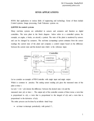
  • 1. Dr.Y.Narasimha MurthyPh.D yayavaram@yahoo.com 1 RTOS APPLICATIONS RTOS find applications in various fields of engineering and technology .Some of them include Control systems, Image processing, Fault Tolerance systems etc. (i).RTOS for control systems Many real-time systems are embedded in sensors and actuators and function as digital controllers. The term plant in the block diagram below refers to a controlled system, for example, an engine, a brake, an aircraft, a patient. The state of the plant is monitored by sensors and can be changed by actuators. The real-time (computing) system estimates from the sensor readings the current state of the plant and computes a control output based on the difference between the current state and the desired state which is the reference input. Let us consider an example of PID Controller with single input and single output Which is common in practice. The analog sensor reading y(t) gives the measured state of the plant at time t. Let e(t) = r (t) − y(t) denote the difference between the desired state r (t) and the measured state y(t) at time t . The output u(t) of the controller consists of three terms: a term that is proportional to e(t), a term that is proportional to the integral of e(t) and a term that is proportional to the derivative of e(t). The entire process can be done by an infinite timed loop  set timer to interrupt periodically with period T ;
  • 2. Dr.Y.Narasimha MurthyPh.D yayavaram@yahoo.com 2  at each timer interrupt, do  do analog-to-digital conversion to get y;  compute control output u;  output u and do digital-to-analog conversion;  end do; Here, we assume that the system provides a timer. Once set by the program, the timer generates an interrupt every T units of time until its setting is cancelled. The length T of time between any two consecutive instants at which y(t) and r (t) are sampled is called the sampling period. T is a key design choice. The behavior of the resultant digital controller critically depends on this parameter. Ideally we want the sampled data version to behave like the analog version. This can be done by making the sampling period small. However, a small sampling period means more frequent control-law computation and higher processor-time demand. We want a sampling period T that achieves a good compromise. In making this selection, two factors are to be considered. The first is the perceived responsiveness of the overall system (i.e., the plant and the controller). Oftentimes, the system is operated by a person (e.g., a driver or a pilot). The operator may issue a command at anytime, say at t . The consequent change in the reference input is read and reacted to by the digital controller at the next sampling instant. This instant can be as late as t + T . Thus, sampling introduces a delay in the system response. The operator will feel the system sluggish when the delay exceeds a tenth of a second. Therefore, the sampling period of any manual input should be under this limit. The second factor is the dynamic behavior of the plant. We want to keep the oscillation in its response small and the system under control. To explain this let us consider a disk drive controller. The plant in this example is the arm of a disk. The controller is designed to move the arm to the selected track each time when the reference input changes. At each change, the reference input r (t) is a step function from the initial position to the final position .In figures below these positions are represented by 0 and 1, respectively, and the time origin is the instant when the step in r (t) occurs. The dashed lines in (a) give the output u(t) of the analog controller and the observed position y(t) of the arm as a function of time. The
  • 3. Dr.Y.Narasimha MurthyPh.D yayavaram@yahoo.com 3 solid lines in the lower and upper graphs give, respectively, the analog control signal constructed from the digital outputs of the controller and the resultant observed position y(t) of the arm. At the sampling rate shown here, the analog and digital versions are essentially the same. The solid lines in (b) give the behavior of the digital version when the sampling period is increased by 2.5 times.
  • 4. Dr.Y.Narasimha MurthyPh.D yayavaram@yahoo.com 4 The oscillatory motion of the arm is more pronounced but remains small enough to be acceptable. However, when the sampling period is increased by five times, as shown in figure (c), the arm requires larger and larger control to stay in the desired position; when this occurs, the system is said to have become unstable. In general, the faster a plant can and must respond to changes in the reference input, the faster the input to its actuator varies, and the shorter the sampling period should be. We can measure the responsiveness of the overall system by its rise time R. This term refers to the amount of time that the plant takes to reach some small neighborhood around the final state in response to a step change in the reference input. In the example in the figure above, a small neighborhood of the final state means the values of y(t) that are within 5 percent of the final value. Hence, the rise time of that system is approximately equal to 2.5. Multirate Systems : A plant typically has more than one degree of freedom. Its state is defined by multiple state variables (e.g., the rotation speed, temperature, etc. of an engine or the tension and position of a video tape). Therefore, it is monitored by multiple sensors and controlled by multiple actuators. One can consider a multivariate (i.e., multi-input/multi-output) controller for such a plant as a system of single-output controllers. Because different state variables may have different dynamics, the sampling periods required to achieve smooth responses from the perspective of different state variables maybe different. [For example, because the rotation speed of a engine changes faster than its temperature, the required sampling rate for RPM (Rotation Per Minute) control is higher than that for the temperature control.] Of course, we can use the highest of all required sampling rates. This choice simplifies the controller software since all control laws are computed at the same repetition rate. However, some control-law computations are done more frequently than necessary; some processor time is wasted. To prevent this waste, multivariate digital controllers usually use multiple rates and are therefore called multirate systems. Many times, the sampling periods used in a multirate system are related in a harmonic way, that is, each longer sampling period is an integer multiple of every shorter period. This multirate controller controls only flight dynamics. The control system on board an aircraft is considerably more complex which typically contains many other equally critical subsystems
  • 5. Dr.Y.Narasimha MurthyPh.D yayavaram@yahoo.com 5 (e.g., air inlet, fuel, hydraulic, brakes, and anti-ice controllers) and many not so critical subsystems (e.g., lighting and environment temperature controllers). So, in addition to the flight control-law computations, the system also computes the control laws of these subsystems. Controllers in a complex monitor and control system are typically organized hierarchically. One or more digital controllers at the lowest level directly control the physical plant. Each output of a higher-level controller is a reference input of one or more lower-level controllers. For example, a patient care system may consist of microprocessor-based controllers that monitor and control the patient’s blood pressure, respiration, glucose, and so forth. There may be a higher-level controller (e.g., an expert system) which interacts with the operator (a nurse or doctor) and chooses the desired values of these health indicators. While the computation done by each digital controller is simple and nearly deterministic, the computation of a high level controller is likely to be far more complex and variable. While the period of a low level control- law computation ranges from milliseconds to seconds, the periods of high-level control-law computations may be minutes, even hours. Figure below shows a more complex example: the hierarchy of flight control, avionics,and air traffic control systems . The Air Traffic Control (ATC) system is at the highest level. It regulates the flow of flights to each destination airport. It does so by assigning to each air craft an arrival time at each metering (or waypoint) en route to the destination: The aircraft is supposed to arrive at the metering fix at the assigned arrival time. At any time while in flight, the assigned arrival time to the next metering fix is a reference input to the on-board flight management system. The flight management system chooses a time-referenced flight path that brings the aircraft to the next metering fix at the assigned arrival time. The cruise speed, turn radius, decent/accent rates, and so forth required to follow the chosen time-referenced flight path are the reference inputs to the flight controller at the lowest level of the control hierarchy. As another example for higher levels of control let us consider a control system of robots that perform assembly tasks in a factory for example. Path and trajectory planners at the second level determine the trajectory to be followed by each industrial robot. These planners typically take as an input the plan generated by a task planner, which chooses the sequence of assembly steps to be performed. In a space robot control system, there may be a scenario planner, which
  • 6. Dr.Y.Narasimha MurthyPh.D yayavaram@yahoo.com 6 determines how a repair or rendezvous function should be performed. The plan generated by this planner is an input of the task planner. Fig: Air traffic/flight control hierarchy An Air Traffic Control (ATC) system is an excellent example for Real-Time Command and Control. The ATC system monitors the aircraft in its coverage area and the environment (e.g, weather condition) and generates and presents the information needed by the operators (i.e., the air traffic controllers). Outputs from the ATC system include the assigned arrival
  • 7. Dr.Y.Narasimha MurthyPh.D yayavaram@yahoo.com 7 times to metering fixes for individual aircraft. As stated earlier, these outputs are reference inputs to on-board flight management systems. Thus, the ATC system indirectly controls the embedded components in low levels of the control hierarchy. In addition, the ATC system provides voice and telemetry links to on-board avionics. Thus it supports the communication among the operators at both levels (i.e., the pilots and air traffic controllers).The ATC system gathers information on the “state” of each aircraft via one or more active radars. Such a radar interrogates each aircraft periodically. When interrogated, an air- craft responds by sending to the ATC system its “state variables”: identifier, position, altitude, heading, and so on. Fig:An architecture of air traffic control system
  • 8. Dr.Y.Narasimha MurthyPh.D yayavaram@yahoo.com 8 The ATC system processes messages from aircraft and stores the state information thus obtained in a database. This information is picked up and processed by display processors. At the same time, a surveillance system continuously analyzes the scenario and alerts the operators whenever it detects any potential hazard (e.g., a possible collision). Again, the rates at which human interfaces (e.g., keyboards and displays) operate must be at least 10 Hz. The other response times can be considerably larger. For example, the allowed response time from radar inputs is one to two seconds, and the period of weather updates is in the order of ten seconds. From the above example, it is clear that a command and control system bears little resemblance to low-level controllers. In contrast to a low-level controller whose workload is either purely or mostly periodic, a command and control system also computes and communicates in response to sporadic events and operators’ commands. Furthermore, it may process image and speech, query and update databases, simulate various scenarios, and the like. The resource and processing time demands of these tasks can be large and varied. Fortunately, most of the timing requirements of a command and control system are less stringent. Whereas a low-level control system typically runs on one computer or a few computers connected by a small network or dedicated links, a command and control system is often a large distributed system containing tens and hundreds of computers and many different kinds of networks. In this respect, it resembles interactive, on-line transaction systems (e.g., a stock price quotation system) which are also sometimes called real-time systems. (ii). RTOS for image processing: Real-time image processing (RTIP) promises to be at the heart of many developments in computer technology: context aware computers, mobile robots, Medical augmented reality and the subject of research — video-based interfaces for human computer interaction. These applications have significant demands not only in terms of processing power: they must achieve real-time, low latency response to their visual input. The modern operating systems provide a wealth of multimedia features which are usually oriented towards the playback or recording of media rather than processing in real time.
  • 9. Dr.Y.Narasimha MurthyPh.D yayavaram@yahoo.com 9 One can think of three types of Real Time Imaging systems. Soft real time Imaging, Firm Real Time Imaging and Hard Real Time Imaging systems. In Soft real-time imaging systems, missed deadlines manifest as performance degradation. For example , the image processing used in an animated cartoon system. Here each cartoon frame is separately processed and only played back in real-time at the end. So, while exceptionally slow processing of each frame might be annoying, it will not affect the end product. Most entertainment systems tend to fall into the category of soft real-time imaging. On the other hand, “firm” real-time imaging systems can tolerate a few missed deadlines. In many imaging systems, for example, a common deadline is that the screen be updated at least 30 times per second. If this deadline is missed frequently, the image will not appear as continuous motion and the system will have failed. However, a small number of missed deadlines are acceptable. But in a “hard” real-time imaging system even one missed deadline can lead to disaster. For example, consider the need to identify an enemy aircraft using an image- matching algorithm within a few milliseconds. Failure to meet that deadline, identify the enemy and destroy it can have catastrophic consequences. This class of real-time imaging systems is the most challenging to build. Multimedia systems are complex real-time imaging systems that incorporate powerful processors, high-speed networks and massive storage devices. Significant research is focused on developing high bus bandwidth and display capability for the vast number of large images that must be processed. For example, until very recently, high resolution real-time could only be obtained using specialized image processing boxes such as Silicon Graphic’s machines. Today, such images can be processed on modestly-high performance PCs. Another real-time imaging concern is in the development of compression and decompression techniques that effectively manage data loss, compression rate, and decompression rate and performance predictability. Different media representations and handling mechanisms are often necessary for real-time processing. The operating system itself must also be capable of efficient, low-latency response and processing. Mac OS X provides a robust operating system with excellent latency performance and a rich multimedia framework that can be applied, with some provisions to RTIP applications. For real time image processing the following provisions are required
  • 10. Dr.Y.Narasimha MurthyPh.D yayavaram@yahoo.com 10 • high resolution, high frame rate video input • low latency video input • low latency operating system scheduling • high processing performance. In the most general terms, image processing attempts to extract information from the outside world through its visual appearance. Therefore adequate information must be provided to the processing algorithm by the video input hardware. Precise requirements will, depend on the algorithm and application but usually both spatial and temporal resolution are important. Broadcast video provides a practical reference point as most cameras provide images in formats derived from broadcast standards regardless of their computer interface (analog, USB etc). Higher resolution in both spatial and temporal sampling is desirable for many applications. Low latency video input: All video input systems have intrinsic sources of latency in their hardware and transmission schemes. Indeed, the relatively sparse temporal sampling (frame rate) typical for video can itself be thought of as a source of latency equal to the frame duration. Higher frame rates therefore allow for lower latency and more responsive RTIP systems. Additional latency occurs in the transmission of video from the camera to the computer interface. The sequential nature of almost all video frame transmission also imposes latency equal to the frame transmission time (which is usually close to the frame duration in order to minimise bandwidth requirements). This applies to digital transmission schemes over USB or Fire wire just as it does to analogue transmission. Low latency operating system scheduling: Once the video signal arrives at the computer it will be processed and passed between a number of software components. These components will depend on the type of video capture hardware in use, but generally and in the minimum case there will be a driver component and an application that performs the image processing. The driver is responsible for receiving the transmission and presenting the video frame as a buffer of pixels and is of course provided by the operating system vendor or hardware vendor. This pixel buffer is then processed by the application which would then typically produce some output for the user or provide information to other application software running on the system.
  • 11. Dr.Y.Narasimha MurthyPh.D yayavaram@yahoo.com 11 The ability of the Real Time operating system to respond to incoming video data and to schedule each of these software components to run as soon as its data are available has a crucial impact on system latency. If no input data is to be lost, buffering (and hence additional latency) must be introduced to cover both lag and any variation in when data is available and when it is passed to the next component. This lag and variation is related to system interrupt latency and scheduling latency. For example the Real Time OS Mac OS X has excellent low latency performance even under heavy system load as evidenced by its reliable behaviour with low latency audio software. High Processing performance: Image processing algorithms are very bandwidth and processor speed intensive. High bandwidth memory architecture, effective caching and high performance processors are necessary for an RTIP platform. Altivec is an important factor in achieving good performance, as image processing algorithms are usually highly parallel and therefore well suited to SIMD optimization. Recent developments in processor hardware architecture [ for ex : in changes in Macintosh hardware architecture] are also very promising for RTIP, in particular the emphasis on memory bandwidth. Video Capture Hardware Video capture hardware performs the vital role of handling the reception of the video signal into the computer and presenting to the processor in a suitable form. Some hardware integrates both camera and digitization functions together, such as the DV video cameras, and USB Webcams. Other systems perform only digitization of an analog video signal provided by an external camera. These devices are then connected to a suitable system bus (PCI, Firewire or sometimes USB). Suitable devices for RTIP must provide high resolution, high frame rate video at low latency. Making the video signal available in an uncompressed format to the image processing software with low CPU overhead is also important. These requirements unfortunately exclude many common video input devices which provide only low quality input or introduce latency through their compression or transmission schemes. USB hardware Both cameras and digitizers are available which use the common and convenient USB for
  • 12. Dr.Y.Narasimha MurthyPh.D yayavaram@yahoo.com 12 communication to the host computer. Unfortunately the low bandwidth of USB 1.1 (11Mbps) is insufficient to convey high resolution video at high frame rate. Most devices are limited to 320x240 pixels at 30fps(frames per second). Some devices provide higher resolution at lower frame rates. Other devices achieve acceptable frame rates and resolution but they must employ a compression scheme such as MPEG to limit their data rate for USB. The MPEG compression schemes not only degrade the visual quality of the incoming signal but usually add latency to the video input stream. USB 2.0 offers sufficient bandwidth for high quality video. PCI hardware The most traditional hardware for RTIP (Real Time Image Processing) is the combination of an analogue camera and a PCI based video digitizer. This approach can offer excellent performance as the video digitizer can perform useful preprocessing and move the video frame buffers via DMA. This style of hardware must be supported by all versions of RTOS.. The Video recording model tries to avoid dropping frames at all costs by adding buffers to the video stream and demanding priority scheduling. An RTIP system would usually prioritize latency over the dropping of frames and therefore introduce as few buffers to the video stream as possible. Furthermore, if critical time deadlines are not being met (such as processing time for other parts of the RTIP system or frame drops due to frame handling taking too long) the behavior of an RTIP scheme will be different to that of a recording scheme. Even if the RTIP system does not require the display of video as part of its output, it is always important to be able to monitor and preview the video stream at various stages of processing. Certain RTOSes like QuickTime includes functions which perform hardware accelerated display of buffer with some pixel formats and appropriate conversions for buffers of many other pixel formats. Real-time imaging design issues: One challenge in designing real-time image processing systems is the high computational intensity of the algorithms involved. For example, image filtering each pixel separately for a 1024 by 1024 pixel display can be very costly in terms of memory requirements and processing time. Typical hardware for real-time imaging applications involves high-performance computers with firmware support for complex instruction sets and algorithmic transformations. However, commercial pixel processors, where one processor is assigned to each pixel, are available and inexpensive. Also, scalable structures, such as the field programmable gate arrays, are increasingly being used. But building systems with highly
  • 13. Dr.Y.Narasimha MurthyPh.D yayavaram@yahoo.com 13 specialized processors is not very easy because there is usually limited expertise with these specialized environments. Also, tool support is generally thin because of overall low market demand. Whatever the hardware platform, many use an object-oriented software approach because of the high-level language support it provides. Such approaches can incur significant performance penalties in terms of memory utilization and time. They can also introduce behavior uncertainty because of garbage collection. For example, in an object-oriented language if every pixel were treated as an object images of faces; analysis of medical images and fingerprints; robotics and artificial intelligence systems. •Multimedia/virtual reality including geometric representations of objects and surfaces; models of scene illumination; geometric representations of image parts; spatial arrangements and image representation; 3D object description; specialized computation techniques. • Algorithms comprising any algorithms for image processing not covered in other areas; multi- image processing; image segmentation. • Software engineering constituting tools, languages and engineering methodologies unique to real-time imaging; imaging aesthetics; cognitive perception and paradigms. (iii). Embedded RTOS for voice over IP(voIP) Voice over IP (VOIP) uses the Internet Protocol (IP) to transmit voice as packets over an IP network. So VOIP can be achieved on any data network that uses IP, like Internet, Intranets and Local Area Networks (LAN). Here the voice signal is digitized, compressed and converted to IP packets and then transmitted over the IP network. It is an advancing technology that is used to transmit voice over the internet or a local area network using internet protocol (IP).This technology provides enhanced features such as low cost compared to the traditional Public Switched Telephone Network (PSTN). VoIP system costs as much as half the traditional PSTN system in the field of voice transmission. This is because of the efficient use of bandwidth requiring fewer long-distance trunks between switches. The voice over internet protocol system is found to be the successful alternative to the traditional PSTN communication system due to its advanced features. The voice signal is processed through
  • 14. Dr.Y.Narasimha MurthyPh.D yayavaram@yahoo.com 14 the internet based network during the communication. The conceptual diagram of VoIP system is shown in Fig.below. The basic steps in derivation of the designed VoIP system are:  The original speech signal is fed in to the system and the speech samples are taken from .  The speech signal is then encoded with G.711a and Speex speech encoders, which is the compressed version of the input signal. G.711a is the standard used for the communication purpose and is a high bit rate Pulse Code Modulation codec. It works at sampling rate of 8 kHz and uses and compresses the 16 bit audio samples into 8bits . The Code Excited Linear Prediction (CELP) Speex codec is an open source codec developed for the packet network and VoIP applications.The Speex supports three different sampling rates narrowband (8 kHz), wideband (16 kHz) and ultra-wideband (32 kHz).  The compressed signal is then packetized into VoIP packets to transfer it to the IP network.  The speech signal is degraded due to the various network impairments including delay, jitter and packet loss during VoIP communications. The network impairments are introduced through the lab WANem emulator .  The degraded VoIP signal is depacketized and then decoded with G.711a and Speex decoders.  The performance is evaluated with Perceptual Evaluation of Speech Quality (PESQ) measurement defined by ITU-T recommendation P.862 . After comparing the degraded
  • 15. Dr.Y.Narasimha MurthyPh.D yayavaram@yahoo.com 15 signal with the original one, the PESQ measurement gives the subjective measurement as Mean Opinion Scores (MOS) value from -0.5 to 4.5.  The VoIP signal is processed through various signal processing algorithms to evaluate the performance of the system. Voice quality in communication systems is influenced by many factors such as packet delay, jitter, packet loss and type & amount of voice compression. Due to these distortion factors, the speech signal is not of very good quality over the VoIP network. Delay is the time taken by the voice to reach from talker’s mouth to the listener’s ear. Round trip delay is the sum of two one- way delays that occur in the user’s call. In VoIP system, the propagation delay is also affected by two additional delays such as packeting delay and the time required for propagating the packet through the network. This varies the propagation delay during the transmission. The variation in the arrival time of the packets at the receiver end leads to jitter, which affects the perceived quality of conversation very badly. The sender is expected to transmit each voice packet at a regular interval. But jitter affects the speech in such a way that all voice packets do not arrive at the right time at the decoder and thus reconstructed speech would not be continuous, at the receiver end. The transmission time of a packet through IP network varies due to queuing effect in the interconnected network. The packet loss is the percentage of the lost packets during the transportation due to various network conditions such as buffer overflow, network congestion etc. The delay and jitter also contribute to the packet losses and these results in harmful effects on the quality of VoIP signal. Due to the real time requirement for interactive speech transmission, it is usually impossible for the receivers to request the sender to retransmit the lost packets. When voice packets do not arrive before their payout time, they are considered as lost and cannot be played when they are received. Even a single lost packet may generate audible distortion in the decoded speech signal. To analyze the effect of packet loss on the quality of the degraded VoIP output, the spectral analysis was performed in time and frequency by using various signal processing algorithms. The real-time establishment scheme assumes that scheduling in the hosts and in the nodes will be deadline-based. Each real-time packet in the node is given a deadline, which is the time by which it is to be serviced. Let di, n be the local delay bound assigned to channel i in node n. A packet
  • 16. Dr.Y.Narasimha MurthyPh.D yayavaram@yahoo.com 16 traveling on that channel and arriving at that node at time to will usually be assigned a node deadline equal to to+di, n . The scheduler maintains at least two queues : one for real-time packets and the other for all other types of packets and all local tasks. The first queue has higher priority, is ordered according to packet deadlines, and served in order of increasing deadlines. The second queue can be replaced by multiple queues, managed by a variety of policies. At channel establishment time, each intermediate node checks whether it will be able to accept packets at the rate declared by the sender. However, malicious users or faulty behavior by system components could cause packets to arrive into the network at a much higher rate than the declared maximum value, 1/x min. This can prevent the satisfaction of the delay bounds guaranteed to other clients of the real-time service. A solution to this problem consists of providing distributed rate control by extending the deadlines of the ‘‘offending’’ packets. The deadline assigned to an offending packet would equal the deadline that packet would have if it had obeyed the xmin constraints declared at connection establishment time. (iv).RTOS for fault tolerant applications : Fault tolerance is the ability to continue operating despite the failure of a limited subset of their hardware or software. So the goal of the system designer is to ensure that the probability of system failure is acceptably small. There can be either hardware fault or software fault, which disturbs the real time systems to meet their deadlines. Real time systems are systems in which there is a guaranty for timely response by the computer to external input. Real time applications have to function correctly even in presence of faults. Fault tolerance can be achieved by either hardware or software or time redundancy. Safety- critical applications have strict time and cost constraints, which means that not only faults have to be tolerated but also the constraints should be satisfied. Deadline scheduling means that the task with the earliest required response time is processed. The most common scheduling algorithms are : Rate Monotonic(RM) and Earliest deadline first(EDF). In soft real-time systems it is more important to economically detect a fault as soon as possible rather than to mask a fault. Examples of soft real-time systems are all kind of airline reservation, banking, and E-commerce applications.
  • 17. Dr.Y.Narasimha MurthyPh.D yayavaram@yahoo.com 17 There are three types of faults: Permanent, intermittent, and transient. A permanent fault does not die away with time, but remains until it is repaired as the affected unit is replaced. This is an intermittent fault cycle between the fault–active and fault benign states. A transient fault dies away after some time. Fault detection can be done either online or offline. Online detection goes on in parallel with normal system operation. Offline detection consists of running diagnostic tests. In order to achieve fault tolerance, the first requirement is that transient faults have to be detected. Several error-detection techniques are there against transient faults: watchdogs, duplication and few others.  Watchdogs: In the case of watchdogs program flow or transmitted data is periodically checked for the presence of errors. In the simplest watchdog scheme, watchdog timer, monitors the execution time of processes, whether it exceeds a certain limit.  Duplication: Duplication is an approach to have multiple processors, which are supposed to put out the same result and compare the results. A discrepancy indicates the existence
  • 18. Dr.Y.Narasimha MurthyPh.D yayavaram@yahoo.com 18 of a fault . There are several other error-detections techniques, e.g. signatures, assertions or the widely-used parity bit check.  Redundancy : Fault tolerance system is to be kept running despite the failure of some of its parts, it must have spare capacity to begin. There are two ways to make a system more resistant to faults. Hardware: this technique relies on adding extra redundant hardware to a system to make it fault tolerant. -Software: this technique relies on duplicating the code, process, or even messages, depending on the context. A typical example of where the above techniques are applied would be the autopilot system on-board a large-sized passenger aircraft. A passenger aircraft typically consists of a central autopilot system with two other backups. This is an example of making a system with two other backups. This is an example of making a system fault tolerant by adding redundant hardware. The two extra systems will not be used unless the main system is completely broken. However, this is not sufficient, since in the event that the main system starts behaving erratically the lives of many people is in danger. The system is therefore also made resistant to faults using software However, such measures are only applied for highly critical systems. In general, hardware redundancy is avoided as far as possible, due to limited resources that are available. Weight of the system, power consumption, and price constraints make it difficult to employ high hardware redundancy to make the system fault tolerant. Software redundancy is therefore, more commonly used to increase fault tolerance of systems. There are few factors that affect the diversity of the multiple versions. The first factor is the requirements specification. A mistake in the specification causes a wrong output to be delivered. A second approach is the programming language. The nature of the language affects the programming style greatly. A third factor is the numerical algorithms that are used. Algorithms implemented to a finite precision can behave quite differently for certain sets of inputs than do theoretical algorithms, which assume infinite precision. A fourth factor is the nature of the tools that are being used; the probability of common-mode failure might increase. A fifth factor is the training and quality of the programmers and the management structure. The major difficulty in software is labor-intensive. Fault Tolerance Techniques
  • 19. Dr.Y.Narasimha MurthyPh.D yayavaram@yahoo.com 19 (i)TMR (Triple Modular Redundancy): Multiple copies are executed and error checking is achieved by comparing results after completion. In this scheme, the overhead is always on the order of the number of copies running simultaneously. (ii) PB (Primary/Backup): The tasks are assumed to be periodic and two instances of each task (a primary and a backup) are scheduled on a uni-processor system. One of the restrictions of this approach is that the period of any task should be a multiple of the period of its preceding tasks. It also assumes that the execution time of the backup is shorter than that of the primary. (iii) PE (Primary/Exception): It is the same as PB method except that exception handlers are executed instead of backup programs. (iv)Primary Backup Fault Tolerance : This is the traditional fault-tolerant approach wherein both time as well as space exclusions are used. The main idea behind this algorithm is that (a) the backup of a task need not execute if its primary executes successfully, (b) the time exclusion in this algorithm ensures that no resource conflicts occur between the two versions of any task, which might improve the schedulability. Disadvantages in this system are that (a) there is no de- allocation of the backup copy, (b) the algorithm assumes that the tasks are periodic (the times of the tasks are predetermined), (c) compatible (the period of one process is an integral multiple of the period of the other process) and execution time of the backup is shorter than that of the primary process. It can be concluded that appropriate use of redundancy is important in Fault Tolerance ,since too much redundancy increases reliability but potentially decreases the schedulability. Too little redundancy decreases reliability but increases schedulability. Also, designing, managing redundancy incurs additional cost, time, and memory and power consumption. Acknowledgement: Thanks are due to Prof.Philip A.Laplante, Prof.Daniel HeckenBerg, Dr.T.R.Gopalkrishnan Nair and Prof.A.Christy Persya without whose papers, the preparation of this material can’t be thought of.