Photoelectric detectors xs

31100 _Ver3.00-EN.fm/2 Schneider Electric
Inductive proximity sensors enable the detection, without contact, of metal
objects at distances of up to 60 mm.
Their range of applications is very extensive and includes : the monitoring of
machine parts (cams, mechanical stops, etc.), monitoring the flow of metal
parts, counting, etc.
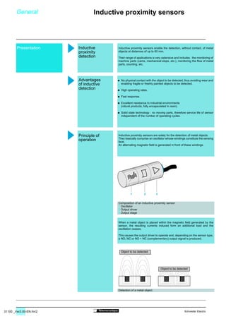
Inductive proximity sensors are solely for the detection of metal objects.
They basically comprise an oscillator whose windings constitute the sensing
face.
An alternating magnetic field is generated in front of these windings.
Composition of an inductive proximity sensor
1 Oscillator
2 Output driver
3 Output stage
When a metal object is placed within the magnetic field generated by the
sensor, the resulting currents induced form an additional load and the
oscillation ceases.
This causes the output driver to operate and, depending on the sensor type,
a NO, NC or NO + NC (complementary) output signal is produced.
Detection of a metal object.
/ No physical contact with the object to be detected, thus avoiding wear and
enabling fragile or freshly painted objects to be detected.
/ High operating rates.
/ Fast response.
/ Excellent resistance to industrial environments
(robust products, fully encapsulated in resin).
/ Solid state technology : no moving parts, therefore service life of sensor
independent of the number of operating cycles.
Presentation
1 2 3
Inductive proximity sensors enable the detection, without contact, of metal
objects at distances of up to 60 mm.
Their range of applications is very extensive and includes : the monitoring of
machine parts (cams, mechanical stops, etc.), monitoring the flow of metal
parts, counting, etc.
Inductive proximity sensors are solely for the detection of metal objects.
They basically comprise an oscillator whose windings constitute the sensing
face.
An alternating magnetic field is generated in front of these windings.
Composition of an inductive proximity sensor
1 Oscillator
2 Output driver
3 Output stage
When a metal object is placed within the magnetic field generated by the
sensor, the resulting currents induced form an additional load and the
oscillation ceases.
This causes the output driver to operate and, depending on the sensor type,
a NO, NC or NO + NC (complementary) output signal is produced.
Detection of a metal object.
/ No physical contact with the object to be detected, thus avoiding wear and
enabling fragile or freshly painted objects to be detected.
/ High operating rates.
/ Fast response.
/ Excellent resistance to industrial environments
(robust products, fully encapsulated in resin).
/ Solid state technology : no moving parts, therefore service life of sensor
independent of the number of operating cycles.
General
Inductive
proximity
detection
Advantages
of inductive
detection
Principle of
operation
Inductive proximity sensors
Object to be detected
Object to be detected

31100 _Ver3.00-EN.fm/3Schneider Electric
,,,,,,,,
0,81 Sn
Sn
2 1
Sensing face
H
The operating zone relates to the area in front of the sensing face in which
the detection of a metal object is certain. The values stated in the
characteristics relating to the various types of sensor are for steel objects of
a size equal to the sensing face of the sensor. For objects of a different
nature (smaller than the sensing face of the sensor, other metals, etc.), it is
necessary to apply a correction coefficient (see page 31100/14).
1 Detection threshold curves
2 “Object detected” LED
Nominal sensing distance (Sn).
The rated operating distance for
which the sensor is designed. It
does not take into account any va-
riations (manufacturing tolerances,
temperature, voltage, etc.).
Real sensing distance (Sr).
The real sensing distance is measured
at the rated voltage (Un) and at rated
ambient temperature (Tn).
It must be between 90% and 110% of
the nominal sensing distance (Sn) :
0.9 Sn ≤ Sr ≤ 1.1 Sn.
Usable sensing distance (Su).
The usable sensing distance is
measured at the limits of the per-
missible variations of the ambient
temperature (Ta) and the supply
voltage (Ub). It must be between
90% and 110% of the real sensing
distance (Sr) :
0.9 Sr ≤ Su ≤ 1.1 Sr.
Assured operating distance (Sa).
This is the operating zone of the
sensor.
The assured operating distance is
between 0 and 81% of the nominal
sensing distance (Sn) :
0 ≤ Sa ≤ 0.9 x 0.9 x Sn.
Square mild steel (Fe 360) plate,
1 mm thick.
The side dimension of the plate is
either equal to the diameter of the
circle engraved on the active surface
of the sensing face or 3 times the
nominal sensing distance (Sn).
The differential travel (H), or hyste-
resis, is the distance between the
pick-up point as the standard metal
target moves towards the sensor
and the drop-out point as it moves
away.
The repeat accuracy (R) is the repeatability of the usable sensing distance
between successive operations. Readings are taken over a period of time
whilst the sensor is subjected to voltage and temperature variations :
8 hours, 10 to 30 °C, Un ± 5 %. It is expressed as a percentage of Sr.
General Inductive proximity sensors
Standard metal target
Operating zone
Sensing distances
Standard metal
target
Differential travel
Repeat accuracy
(Repeatability)
Sa
=
H = course différentielle
Terminology
Su max.
Sr max.
Sn
Sr min.
Su min.
Output
ON
Output
OFF
Sr max. + H
Sn + H
Su max. + H
Sr min. + H
Su min. + H
Certain detection
Assured operating
distance
Sensing
distance
Drop-out point
Pick-up point
Frontal approach
Standard metal target

BU
BN
–/+
+/–
BU
BN
BU
BN
BU
BK
BN
PNP
+
–
+
–BU
BK
BN
NPN
BU
WH (NC)
BK (NO)
BN
PNP
+
–
+
–BU
BK (NO)
WH (NC)
BN
NPN
BK
WH
BN (NO), BU (NC)
BU (NO), BN (NC)
BN (NO), BU (NC)
BU (NO), BN (NC)
PNP
+
–
+
–
WH
BK
NPN
XS
XS
XS
Corresponds to a proximity sensor
whose output (transistor or thyristor)
changes to the closed state when an
object is present in the operating
zone.
whose output (transistor or thyristor)
changes to the open state when an
object is present in the operating
zone.
with 2 complementary outputs, one
of which opens and one of which
closes when an object is present in
the operating zone.
/ Not polarity conscious, connections
to + and – immaterial.
/ Protected against overload and
short-circuit.
/ Not protected against overload or
short-circuit.
/ 20…264 V supply, either or $.
/ Certain models protected against
overload and short-circuit.
/ Protected against reverse supply
polarity.
short-circuit.
polarity.
short-circuit.
polarity.
short-circuit.
Output signal
(contact logic)
2-wire type
3-wire type
4-wire type,
complementary outputs
gr
4-wire type,
multifunction,
programmable
NO
NC
NO + NC
complementary
outputs
2-wire $
non polarised
NO or NC output
2-wire
NO or NC output
2-wire 7
NO or NC output
3-wire $
NO or NC output
PNP or NPN
4-wire $
NO and NC
PNP or NPN
4-wire $
NO or NC,
PNP or NPN
Outputs and wiring

2-wire connection
3-wire connection
+
–S I
+
–
+
–
S I
These proximity sensors convert the
approach of a metal object towards
the sensing face into a current
variation which is proportional to the
distance between the object and the
sensing face.
2 models available :
/ Dual voltage : $ 24…48 V
/ Single voltage : $ 24 V
Output 0-16 mA for 3-wire
connection and 4-20 mA for 2-wire
connection
The proximity sensors conforming
to NAMUR (DIN 19234) recommenda-
tions are electronic devices whose
current consumption is altered by the
presence of a metallic object within the
sensing zone.
Their small size makes them
suitable for various applications in
many sectors, notably :
/ Intrinsically safe
/ Non intrinsically safe
Factory fitted moulded cable, good protection against splashing liquids.
Example : machine tool applications.
Ease of installation and maintenance.
Flexibility, cable runs to required length.
For characteristics of the various types of output, wiring precautions and terminology, see pages 31100/15 to 31100/
18.
Output 0-10 mA for 3-wire
connection, and 4-14 mA for 2-
wire connection.
(hazardous areas).
Sensors used with an NY2 intrin-
sically safe relay/amplifier or a
compatible solid state input which
is suitably approved for intrinsi-
cally safe applications.
(normal safe areas).
Sensors used with an XZD power
supply/amplifier unit or a compa-
tible (DIN 19234) solid state input
amplifier.
Analogue type
NAMUR type
Pre-cabled
Connector
Screw terminals
Specific output signals
Connection methods
Additional information
regarding outputs
Outputs and wiring

LED indicators
2
1
1
2
1
2
1
2
1
2
All Telemecanique brand inductive proximity sensors incorporate an output
state LED indicator.
Output LED function table
Certain block type XS7, XS8, XSD inductive proximity sensors incorporate a
supply LED, in addition to the output LED.
This provides instant verification of the supply state of the sensor .
This LED, complementary to the output LED, flashes in the event of a short-
circuit occurring on the load side of the sensor.
It remains in the flashing state until the supply to the sensor is removed and
the short-circuit rectified.
This feature is particularly useful when switching inductive loads, which are
prone to short-circuits.
The short-circuit LED is incorporated in the following 2-wire type and $
short-circuit protected sensors : Ø 18 mm cylindrical type, Ø 30 mm cylindri-
cal type and XSD block type.
No object present
Object present
Short-circuit
Short-circuit LED function table
NO output NC output
No object present
LED
Output state
Object present
LED
Output state
NO output NC output
1 Output LED
2 Short-circuit LED
General
Output LED
Supply LED
Short-circuit LED
Specific functions

Output signal time delay
1
0
1
0
T T
t
t
t
t
1
0
1
0
T
t
t
t
t
Block type XSC and XSD sensors incorporate a potentiometer adjusted 1 to
20 second output time delay.
The outputs of these sensors are programmable (by links) and any of the
following configurations are possible :
/ NO output contact - time delay when an object enters the operating zone,
/ NC output contact - time delay when an object enters the operating zone,
/ NO output contact - time delay when an object leaves the operating zone,
/ NC output contact - time delay when an object leaves the operating zone.
The time delay is triggered as the object enters the operating zone and the
output contact changes state only if the object is still present after the preset
time (T) has elapsed.
Application example : monitoring the flow of metal parts on a conveyor belt.
Time that object is present in the operating zone
The time delay is triggered as the object leaves the operating zone and the
output contact changes state only if the preset time delay (T) elapses before
another object enters the operating zone.
Application example : monitoring for missing metal parts on a conveyor belt.
Time that object is present in the operating zone
Specific functions
Object present in
operating zone
Elapsed time delay
NO output contact
NC output contact
Object present in
operating zone
Elapsed time delay
NO output contact
NC output contact
Principle
Time delay when
object enters
operating zone
Time delay when
object leaves
operating zone

Rotation monitoring
1
0
T (1)
t
t
Fc
Fr
Sensors of the type generally known as “rotation monitoring” compare the
passing speed of metal targets to an internal preset value.
The trajectory of the target objects can either be rotary or linear.
The moving part to be monitored is fitted with metal targets, aligned for
detection by the sensor.
The impulse frequency Fc generated by the moving part to be monitored is
compared with the frequency Fr preset on the sensor.
The output of the sensor is in the closed state for Fc Fr and in the open
state for Fc Fr.
Note : Following “power-up” of the sensor, the “rotation monitoring” function
is subject to a start-up delay of 9 seconds in order for the moving part to run
up to speed.
(Sensors without this feature or with a delay reduced to 3 seconds are also
available on request).
Adjustment of Fr
(1) Start-up time delay (contact closed during start-up period)
Operating curve
Detecting :
/ underspeed,
/ slip,
/ coupling breakage,
/ overload.
Example : coupling breakage detection.
Specific functions
Principle
Operation
Applications
Output
contact
Fr adjustment potentiometer
Metal target
Non metallic material

Features of the
various models
3 Sn 3 Sn
3 Sn
2 Sn
e (mm)
h(mm)
General
Cylindrical type
- fast installation and setting-up,
- pre-cabled or connector output,
- small size facilitates mounting in
locations with restricted access.
Interchangeability, provided by
indexed fixing bracket. When
assembled, becomes similar to a
block type sensor.
Block type
- direct interchangeability, without
the need for readjustment,
- output terminals, providing connection
flexibility,
- robustness.
Sensors suitable for flush
mounting
- no lateral effect, but
- reduced sensing distance.
Sensors not suitable for flush
mounting
- sensing distance greater than that
for flush mountable models, but
- space required around the sensor to
eliminate the effects of surrounding
metal.
/ Standardflushmountable types :
/ Standard non flush mountable
typesandincreasedrangetypes:
Standard model Increased sensing range model
e = 0, h = 0
- Ø 6.5, 8 12 mm e = 0, h = 0
- Ø 18 mm if : h = 0, e ≥ 5
e = 0, h ≥ 3
- Ø 30 mm if : h = 0, e ≥ 8
e = 0, h ≥ 4
Non
ferrous
or
plastic
material
Types of case
Suitability for flush
mounting in metal
Sensors suitable
for flush mounting
Sensors not
suitable for flush
mounting
Mounting in
conjunction with
fixing bracket
Mounting and installation precautions
Mounting cylindrical
type sensors on metal
supports
Metal
Metal
MetalMetal
Metal
Metal
Detected objectDetected object
Detected object
Indexed fixing bracket
Short case Form A case
Form C Form D

Mounting side by side, e ≥ 2 Sn
Mounted face to face, e ≥10 Sn
1,5a
1,5 a
a
3 Sn
a
a
1,5 a
3Sn
1,5a
2 a
2a
a
2 a
2a
3 Sn
a
a
2 a
2 a
3Sn
e
e
Mounting side by side, e ≥ 2 Sn
Mounted face to face, e ≥ 10 Sn
Mounting in the vicinity of metal masses, on one or more sides simultaneously.
Mounting in an angle section
Mounting in a U section
Two sensors mounted too close to
each other are likely to lock in the
“detection” state, due to interference
between their respective oscillating
frequencies.
To avoid this condition, minimum
mounting distances given for the
sensors should be adhered to.
For applications where the minimum recommended mounting distances for
standard sensors cannot be achieved, it is possible to overcome this
restraint by mounting a staggered frequency sensor adjacent or opposite to
each standard sensor.
For information on staggered frequency sensors, please consult your
Regional Sales Office.
Correct mounting Not to be recessed Not to be mounted
mounted adjacent to an angle
Mounting block type
sensors on metal
supports
Mounting distance
between sensors
Metal Metal Metal
Metal Metal Metal
Metal Metal Metal
Sensing
face
Sensing
face
Sensing
face
Metal Metal Metal
Metal Metal Metal
Sensing
face
Sensing
face
Sensing
face
Sensors suitable
for flush mounting
Sensors not
suitable for flush
mounting
Standard sensors
Staggered
frequency sensors

1
2
1
2
1 Insert the sensor into the bracket.
2 Secure sensor in fixing bracket using screw V.
3 The sensor is now rigidly clamped in the fixing bracket.
Adjust the bracket/sensor assembly to ensure correct detection and
positively secure the assembly using fixing screws F.
The proximity sensor is positively indexed in position. If, for any reason, it is
necessary to change the sensor :
- loosen screw V and remove sensor,
- insert the new sensor until it is against the stop. On tightening screw V, the
new sensor will be indexed into the same position as the previous sensor.
Plug-in body sensors enable mechanical separation of the part containing all
the necessary electronics and the base part comprising the electrical
connections and fixing points.
This feature considerably reduces maintenance time in the event of a sensor
being replaced, since only the electronic part need be replaced. The base
part remains fixed in position, without the need of remaking the electrical
connections or adjusting the settings.
Sensors type XSB, XS7, XS8 and XSD feature a plug-in body.
In addition, sensors type XS7 and XS8 incorporate a 5 position turret
head. The head of the sensor can be rotated laterally throughout the 4 side
detection quadrants or turned vertically for end detection.
Maximum tightening torque for the various sensor case materials
Consider the use of a protective sleeve and CNOMO adaptor.
Brass Brass Stainless Plastic
steel
Diameter Short case Form A Form A All
of sensor model model model models
Ø 5 mm 1.6 1.6 2 –
Ø 8 mm 5 5 9 1
Ø 12 mm 6 15 30 2
Ø 18 mm 15 35 50 5
Ø 30 mm 40 50 100 20
Torque indicated in N.m
1
2 3
1 Part containing sensor electronics
2 Base comprising electrical
connections and fixing points
1 CNOMO adaptor
2 Protective sleeve
Screw VScrew F
Screw F
Mounting cylindrical
type sensors using
fixing bracket
Plug-in body
Turret head
Tightening torque for
cylindrical type sensors
Protection of
connecting cable

All Telemecanique brand proximity sensors conform to the standard IEC 60947-5-2.
/ Operating temperature range of sensors : - 25…+ 70 °C.
/ Storage temperature range of sensors : - 40…+ 85 °C.
Owing to the very wide range of chemicals encountered in modern industry, it is very difficult to give general guidelines
common to all sensors.
To ensure lasting efficient operation, it is essential that the chemicals coming into contact with the sensors will not
affect their casings and, in doing so, prevent their reliable operation.
Cylindrical type metal case sensors XS1-N, XS2-N and XS1-M, XS2-M offer very good resistance to oils in general,
salts, essences and hydrocarbons. Also, sensor models XS1-M and XS2-M are particularly well adapted to severe
environments such as machine-tool applications.
Note : The cable used conforms to the standard NF C 32-206 and the recommendations of CNOMO E 03-40-150 N.
Cylindrical type plastic case sensors XS3 and XS4 offer an excellent overall resistance to :
- chemical products such as salts, haliphactic and aromatic oils, essences, acids and diluted bases. For alcohols,
ketones and phenols, preliminary tests should be made relating to the nature and concentration of the liquid.
- agricultural and food industry products such as animal or vegetable based food products (vegetable oils, animal fat,
fruit juice, dairy proteins, etc.).
The sensors are tested in accordance with the standard IEC 60068-2-27, 50 gn, duration 11 ms.
The sensors are tested in accordance with the standard IEC 60068-2-6, amplitude ± 2 mm, f = 10…55 Hz,
25 gn at 55 Hz.
Please refer to the reference/characteristic pages for the various sensors.
IP 67 : Protection against the effects of immersion, tested in accordance with the standard IEC 529. Sensor immersed
for 30 minutes in 1 m of water.
No deterioration in either operating or insulation characteristics is permitted.
IP 68 : Protection against the effects of prolonged immersion. The test conditions are subject to agreement between
the manufacturer and the user.
Example : Machine-tool applications or other machines frequently drenched in cutting fluids.
Inductive proximity sensors have “TC” protective treatment as standard.
Exceptions :
- Increased range sensors : - 25…+ 50 °C,
- Plastic case cylindrical type sensors (XS3-P and XS4-P) : - 25…+ 80 °C,
- Metal case cylindrical type form A sensors (XS1-M and XS2-M) : - 25…+ 80 °C.
Conformity to standards
Resistance to
temperature
Resistance to
chemicals in
the environment
Resistance to shock
Resistance to vibration
Degree of protection
Protective treatment
Standards and certifications
Parameters related to the environment

Proximity sensors type XS1, XS2, XS3, XS4, XSE, XS7 and XS8 are tested in accordance with the recommendations
of the standard IEC 60947-5-2.
/ $ sensors : level 3 immunity except Ø 4 mm and Ø 5 mm (level 2).
/ and 7 sensors : level 4 immunity.
IEC 61000-4-2
Level 3 : 8 kV
Level 4 : 15 kV
/ $, and 7 sensors : level 2 or level 3 immunity.
IEC 61000-4-3
Level 2 : 3 V/metre
Level 3 : 10 V/metre
/ $ sensors : level 3 immunity.
/ and 7 sensors : level 4 immunity except Ø 8 mm (level 2).
/ Models with increased sensing range : level 2 immunity (at I = 50 mA).
IEC 61000-4-4
/ $, and 7 sensors : level 3 immunity except Ø 8 mm and smaller
models : level 1 kV.
IEC 60947-5-2
Level 3 : 2.5 kV
Electrical insulation conforming to the standards IEC 61140 and NF C 20-030
concerning means of protection against electrical shocks.
/ Cylindrical type sensors
/ Block type sensors
Level 3 : 1 kV
Level 4 : 2 kV
Standard version : UL, CSA except sensors with integral connector type XS/-////////LD,
XS/-////////LA, XS/-////////C and XS/-////////T.
The certifications pertaining to the various block type models are listed on their respective characteristic pages.
General
Resistance to
electromagnetic
interference
Dielectric strength
Insulation
Product certifications
Standards and certifications
Parameters related to the environment
Electrostatic
discharges
Radiating
electromagnetic
fields
(electromagnetic
waves)
Fast transients
(motor start/stop
interference)
Impulse voltages
Class 2 devices
)

Correction coefficients
to apply to the assured
sensing distance
Sa
Kθ x Km x Kd x Kt
4.5
0.98 x 0.9 x 1 x 0.9
-25 0 20 50 70
1,1
0,9
1
Km
0,5
CuAU4GUZ33A37type
304
type
316
Steel Brass Alumin.Copper Iron Bronze
Magnetic
Stainless steel Lead
1Km
0,9
0,8
0,7
0,6
0,5
0,4
0,3
0,2
0,2 0,4 1
0,1
0,1 0,3 0,5 1,5
4 Sn3 Sn2 SnSn
1Kd
0,9
0,8
0,7
0,6
0,5
0,4
0,3
0,2
0,1
In practice, most target objects are generally made of steel and are of a size equal to, or greater, than the sensing
face of the proximity sensor.
To calculate the sensing distance for other application conditions the following parameters, which affect the sensing
distance, must be taken into account :
Note : The curves indicated below are purely representative of typical curves. They are given as a guide to the
approximate usable sensing distance of a proximity sensor for a given application.
Apply a correction coefficient Kθ, determined from the curve shown above.
Apply a correction coefficient Km, determined from the diagram shown
above.
Typical curve for a copper object used with a Ø 18 mm cylindrical sensor.
Special case for a very thin object made from a non ferrous metal.
Typical curve for a steel object used with a Ø 18 mm cylindrical sensor.
When calculating the
sensing distance for the
selection of a sensor, make
the assumption that Kd = 1.
Apply a correction coefficient Kd, determined from the curve shown
above.
In all cases, apply the correction coefficient Kt = 0.9.
Example 1 : correction of the sensing distance of a sensor
Proximity sensor XS7-C40FP260 with nominal sensing distance Sn = 15 mm.
Ambient temperature variation 0 to + 20 °C.
Object material and size : steel, 30 x 30 x 1 mm thick.
The assured sensing distance Sa can be determined using the formula :
Sa = Sn x Kθ x Km x Kd x Kt = 15 x 0.98 x 1 x 0.95 x 0.9, i.e. Sa = 12.5 mm.
Example 2 : selecting a sensor for a given application
Application characteristics :
- object material and size : iron (Km = 0.9), 30 x 30 mm,
- temperature : 0 to 20 °C (Kθ = 0.98),
- object detection distance : 3 mm ± 1.5 mm, i.e. Sa max. = 4.5 mm,
- assume Kd = 1.
One possible choice is a Ø 18 mm cylindrical non flush mountable sensor, type XS2-M18PA370 (Sn = 8 mm).
A sensor must be selected for which Sn ≥ = , i.e. Sn ≥ 5.7 mm.
Sensing distance correction coefficients
Calculation examples
Temperature °C
Variations in
ambient
temperature
Different types of
object material
Size of the object
to be detected
Variation of
supply voltage
Thickness of object in mm
Side lengths of object in mm

Ir
MA
XU
Ud
V
XU
RrRa
t
Sensor operational at state 1
Supply voltage U on
Sensor at state 0
Residual current (Ir)
The residual current (Ir) corresponds to the current flowing through the
sensor when in the “open” state.
Characteristic of 2-wire type proximity sensors.
Voltage drop (Ud)
The voltage drop (Ud) corresponds to the voltage at the sensor's terminals
when in the “closed” state.
(Value measured at nominal current rating of sensor).
Characteristic of 2-wire type proximity sensors.
First-up delay
The time (t) between the connection of the power supply to the proximity
sensor and its fully operational state.
Delays
/ Response time (Ra) :
/ Recovery time (Rr) :
Check that the voltage limits of the proximity sensor are compatible with the
rated voltage of the a.c. supply used.
d.c. source : Check that the voltage limits of the proximity sensor and the
acceptable level of ripple, are compatible with the supply used.
a.c. source (comprising transformer, rectifier, smoothing capacitor) :
The supply voltage must be within the operating limits specified for the
proximity sensor.
Where the voltage is derived from a single-phase a.c. supply, the voltage
must be rectified and smoothed to ensure that :
- The peak voltage of the d.c. supply is lower than the maximum voltage
rating of the proximity sensor.
Peak voltage = nominal voltage x √2
- The minimum voltage of the d.c. supply is greater than the minimum
voltage rating of the proximity sensor, given that :
∆V = (I x t) / C
∆V = maximum ripple : 10 % (V),
I = anticipated load current (mA),
t = period of 1 cycle (10 ms full wave rectified for a 50 Hz supply frequency),
C = capacitance (µF).
As a general rule, use a transformer with a lower secondary voltage (Ue)
than the required d.c. voltage (U).
Example :
18 V to obtain $ 24 V,
36 V to obtain $ 48 V.
Fit a smoothing capacitor of 400 µF minimum per proximity sensor, or 2000 µF
minimum per Ampere required.
Note : Certain models have increased operating limits.
/ short case models XS1-N, XS2-N, XS3-P, XS4-P (10…38 V) :
can be supplied from full wave rectified and smoothed 24 V,
/ form A case 3-wire type models XS1-M, XS2-M, XS3-P, XS4-P (10…58 V):
can be supplied from full wave rectified 24 V.
The time delay between entry of an object (standard metal target) into
the operating zone of the proximity sensor and the subsequent change
of output state.
This parameter limits the speed and size of the object.
The time delay between an object (standard metal target) leaving the
operating zone, in which it is being detected, and the subsequent change
of output state.
This parameter limits the interval between successive objects.
Terminology
Power supplies
Specific aspects of electronic sensors
Proximitysensors
for a.c. circuits
( and 7 models)
Proximitysensors
for d.c. circuits

Types of output
Connection in series
/
/
PNP
+
–
NPN
+
–
U supply
n sensors
These proximity sensors are wired in series with the load to be switched.
Because of this they are subject to :
- a residual current (in the open state),
- a voltage drop (in the closed state).
For polarised (polarity conscious) $ proximity sensors, the supply polarities
must be observed.
For non polarised (not polarity conscious) $ proximity sensors, the supply
polarity and load connections to the + or - sides are immaterial.
Advantages :
- The proximity sensors can be wired in the same way as mechanical limit
switches.
- For and 7 models, they can be connected to either positive (PNP) or
negative (NPN) logic inputs. No risk of incorrect connections.
But :
Check the possible effects of residual current and voltage drop on the input
device being controlled (pick-up and drop-out thresholds).
These proximity sensors comprise 2 wires for the d.c. supply and a third wire
for transmission of the output signal.
- PNP type : switching the positive side to the load,
- NPN type : switching the negative side to the load.
The programmable, universal sensors provide a choice of function, either :
PNP/NO, PNP/NC, NPN/NO or NPN/NC.
Note : Connection can only be made to a single load. Also, it is imperative
that a discharge diode be incorporated when using an inductive load.
The output LED indicator is wired for NPN operation (output ON : LED
illuminated, output OFF : LED off). Therefore, for PNP operation the LED
signalling is reversed.
Advantages :
- Programmable output signal, no residual current, low voltage drop.
- NO + NC versions, for solid state input coincidence control (4-wire type).
- Programmable models, reduced stock levels.
But :
Certain models must only be used with their designated PNP or NPN type of
logic input.
The following points should be
taken into account :
/ Series wiring is only possible
using sensors with wide voltage
limits.
/ When in the open state, each
sensor will share the supply
voltage, i.e. :
(based on the assumption that
each sensor has the same residual
current value).
U sensor and U supply must
remain within the sensor’s voltage
limits.
/ If only one sensor in the circuit is
in the open state, it will be
supplied at a voltage almost
equal to the supply voltage.
/ When in the closed state, a small
voltage drop is present across
each sensor. The resultant loss of
voltage at the load will be the sum
of the individual voltage drops
and therefore, the load voltage
should be selected accordingly.
U sensor =
2-wire type
3-wire type
2-wire type
proximity sensors
Electrical installation of electronic sensors
General

This connection method is not
recommended.
Correct operation of the sensors
cannot be assured and, if this
method is used, tests must be made
before installation. The following
points should be taken into account :
/ Sensor 1 carries the load current
in addition to the no-load current
consumption values of the other
sensors connected in series. For
certain models, this connection
method is not possible unless a
current limiting resistor is used.
/ When in the closed state, each
sensor will produce a voltage drop
and, therefore, the load voltage
should be selected accordingly.
/ As sensor 1 closes, sensor 2 will
not operate until a certain time “T”
has elapsed (corresponding to the
first-up delay) and likewise for the
following sensors in the sequence.
/ “Flywheel” diodes should be
used when the load being swit-
ched is inductive.
The following points should be taken
into account (2 and 3-wire types) :
/ When the mechanical contact is
open, the sensor is not supplied.
/ When the contact closes, the
sensor will not operate until a
certain time “T” has elapsed
(corresponding to the first-up
delay)
The use of proximity sensors
wired in parallel, either between
themselves or together with
mechanical contacts, is not
recommended.
Should one of the sensors be in the
closed state, the sensor in parallel
will be “shorted-out” and no longer
supplied. As the first sensor passes
into the open state, the second
sensor will become energised and
will be subject to its first-up delay.
The configuration is only permissible
where the sensors will be working
alternately.
This method of connection can lead
to irreversible damage of the units.
No specific restrictions.
The use of a “flywheel” diodes is
recommended when an inductive
load (relay) is being switched.
3-wire type
proximity sensors
Wiring sensor
with mechanical
contact
2-wire type
proximity sensors
3-wire type
proximity sensors
Connection in series
(continued)
Connection in parallel

1
2
1
2
– R
– C

No limitation up to 200 m or up to a line capacitance of ≤ 0.1 µF (characteristics
of sensor remain unaffected). It is, however, advisable to take into account
voltage drop on the line.
The proximity sensors are immune to electrical interference encountered in
normal industrial conditions.
Where extreme conditions of electrical “noise” could occur (large motors, spot
welders, etc.), it is advisable to protect against transients in the normal way:
- suppress interference at source,
- limit the length of the cable,
- separate power and control wiring from each other,
- smooth the supply,
- use twisted and screened cable pairs for output signals.
In the event of machine or installation repairs (using an arc welder, for
example), disconnect the proximity sensor.
l
The level of dust and damp protection depends on how carefully the screws,
seals, cable glands, blanking plugs, etc. have been tightened.
To ensure efficient dust and damp protection, use the correct diameter cable
for the cable gland used.
2-wire type proximity sensors cannot be connected directly to an a.c.
supply.
This would result in immediate destruction of the proximity sensor and
considerable danger to the user.
An appropriate load (refer to the instruction sheet supplied with the sensor)
must always be connected in series with the proximity sensor.
At switch-on, it is necessary to limit (by resistor) the charging current of the
capacitive load C.
The voltage drop in the sensor can also be taken into account by subtracting
it from the supply voltage for calculation of R.
R =
If the load comprises an incandescent lamp, the cold state resistance can be
10 times lower than the hot state resistance. This can cause very high
current levels on switching.
Fit a pre-heat resistance in parallel with the proximity sensor.
R = x 10
U = supply voltage
P = lamp power
1 Control cable
2 Power cable
Cable gland Diameter of cable
Ø min. Ø max.
7 mm plastic 3.5 6
9 mm plastic 6 8
11 mm plastic 8 10
13 mm plastic 10 12
U (supply)
I max. (sensor)
U2
P
Wiring advice
a.c. supply
Capacitive load
(C 0.1 µF)
Load comprising an
incandescent lamp
Length of cable
Separation of
control and power
circuit wiring
Dust and damp
protection of
cable glands

Check that the proximity sensor is compatible with the supply being used.
Check the load current characteristics :
- if load current I ≥ nominal current, a relay should be interposed between the
sensor and the load,
- if I ≤ nominal current, check for wiring faults (short-circuit).
In all cases, a “quick-blow” fuse should be fitted in series with the proximity
sensor.
Verify that the wiring conforms to the wiring shown on the proximity sensor
label or instruction sheet
Check that the proximity sensor is compatible with the supply ($ or ).
Check that the supply voltage is within the voltage limits of the sensor.
Remember that with rectified, smoothed supply : U peak = U rms x .
Observe the wiring advice shown on page 31100/18.
Refer to the instruction sheet supplied with the proximity sensor. For sensors
with adjustable sensitivity, reduce the sensing distance.
Check that the supply voltage is within the voltage limits of the sensor.
Ensure that any d.c. supplies, when derived from rectified a.c., are correctly
smoothed (C ≥ 400 µF).
Separate a.c. power cables and d.c. low level cables.
Where very long distances are involved, use suitable cable : screened and
twisted pairs of the correct cross-sectional area.
Position the sensors as far away as possible from any sources of interference.
Check the suitability of the proximity sensor for the object to be detected.
If necessary, select a proximity sensor with a higher switching frequency.
Eliminate sources of radiated heat, or protect the proximity sensor casing
with a heat shield.
Problem Possible causes Remedy
Output stage faulty or the
short-circuit protection has
tripped
Wiring error
Supply fault
Eletromagnet interference
Influence of surrounding metal
Effect of interference on the supply
lines
Response time of the sensor too
slow for the particular object being
detected
Influence of high temperature
Fast trouble shooting guide
The sensor’s output will not
change state when an object
enters the operating zone
False or erratic operation, with or
without the presence of an object
in the operating zone

Photoelectric detectors xs

Recommended

Recommended

More Related Content

What's hot

What's hot (19)

Similar to Photoelectric detectors xs

Similar to Photoelectric detectors xs (20)

More from yared seifu

More from yared seifu (9)

Recently uploaded

Recently uploaded (20)

Photoelectric detectors xs