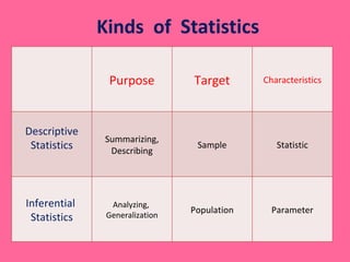
Kinds  of  Statistics Purpose Target Characteristics Descriptive Statistics Summarizing, Describing Sample Statistic Inferential  Statistics Analyzing,  Generalization Population Parameter
 
 
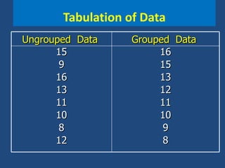
Tabulation of Data Ungrouped  Data  Grouped  Data  15 9 16 13 11 10 8 12 16 15 13 12 11 10 9 8
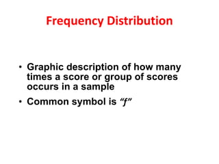
Frequency Distribution Graphic description of how many times a score or group of scores occurs in a sample Common symbol is  “f”
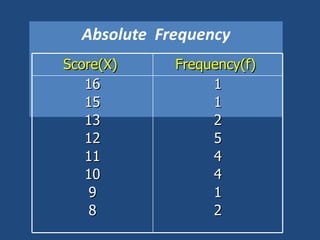
Absolute  Frequency Score(X)  Frequency(f)  16 15 13 12 11 10 9 8 1 1 2 5 4 4 1 2
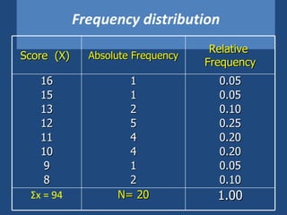
Frequency distribution Score  (X)  Absolute Frequency Relative  Frequency 16 15 13 12 11 10 9 8 1 1 2 5 4 4 1 2 0.05 0.05 0.10 0.25 0.20 0.20 0.05 0.10 Σ x = 94 N= 20 1.00
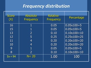
Frequency distribution Score  (X)  Absolute Frequency Relative  Frequency Percentage 16 15 13 12 11 10 9 8 1 1 2 5 4 4 1 2 0.05 0.05 0.10 0.25 0.20 0.20 0.05 0.10 0.05x100=5 0.05x100=5 0.10x100=10 0.25x100=25 0.20x100=20 0.20x100=20 0.05x100=5 0.10x100=10 Σ x = 94 N= 20 1.00 100
Cumulative  Frequency Cumulative frequency distribution  is a graphic depiction of the how many times groups of scores appear in a sample Common symbol is “ cf ” “ cf “ is used to compute percentile scores
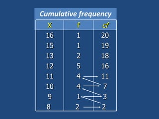
Cumulative frequency X f cf 16 15 13 12 11 10 9 8  1 1 2 5 4 4 1 2  20 19 18 16 11 7 3 2
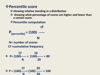
Percentile score  showing relative standing in a distribution showing what percentage of scores are higher and lower than a certain score. Percentile computation    cf P (percentile)  = (100)  ----- N N= number of scores   Cf =cumulative frequency Cf  16 P= (100)-----   =  (100)------ = 80  N  20  Cf  20 P = (100)-----= (100) ------ = 100 N  20
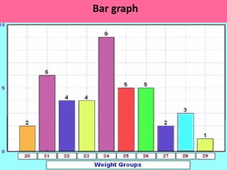
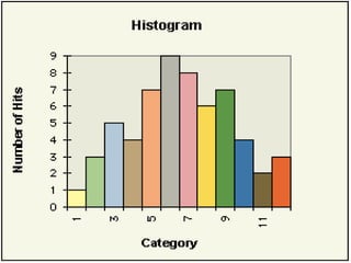
Bar graph
 
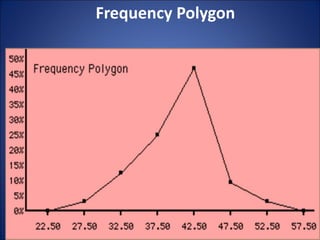
Frequency Polygon
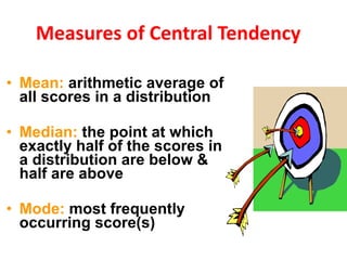
Measures of Central Tendency Mean:  arithmetic average of all scores in a distribution Median:  the point at which exactly half of the scores in a distribution are below & half are above Mode:  most frequently occurring score(s)
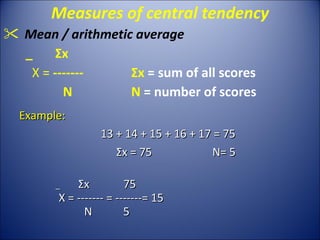
Measures of central tendency Mean / arithmetic average _  Σ x  X =  ------- Σ x  = sum of all scores   N  N  = number of scores Example: 13 + 14 + 15 + 16 + 17 = 75 Σ x = 75 N= 5 _  Σ x  75   X = -------  =  -------= 15 N   5
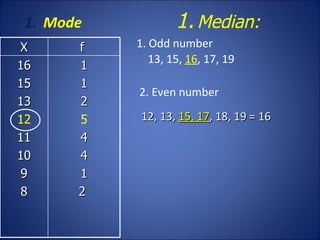
Mode 1. Odd number 13, 15,  16 , 17, 19   2. Even number 12, 13,  15, 17 , 18, 19  =  16 Median:  X f  16 15 13 12 11 10 9 8 1 1 2 5 4 4 1 2
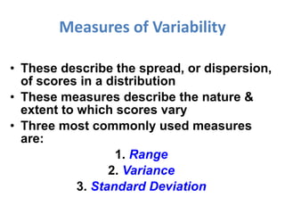
Measures of Variability These describe the spread, or dispersion, of scores in a distribution These measures describe the nature & extent to which scores vary Three most commonly used measures are: 1.  Range 2.  Variance 3.  Standard Deviation
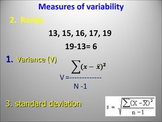
Measures of variability Range 13, 15, 16, 17, 19   19-13= 6 Variance (V)   V   =------------- N -1 3. standard deviation
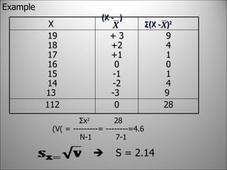
Example   Σ x 2  28     (V (  = ---------= --------=4.6   N-1  7-1   S = 2.14 X  (X -  )   Σ (X -  ) 2 19 18 17 16 15 14 13  + 3 +2 +1 0 -1 -2 -3  9 4 1 0 1 4 9  112 0 28
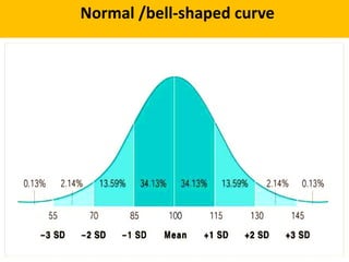
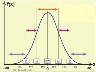
Normal /bell-shaped curve
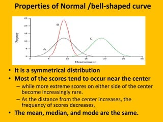
Properties of Normal /bell-shaped curve It is a symmetrical distribution Most of the scores tend to occur near the center while more extreme scores on either side of the center become increasingly rare.  As the distance from the center increases, the frequency of scores decreases.  The mean, median, and mode are the same.
Normal Probability Curve Describes an expected distribution of scores in a population or sample More than 2/3 of scores cluster in the middle of the curve Scores that are extremely high or low are sometimes called outliers Shaped like a bell
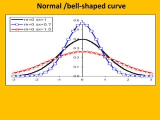
Normal /bell-shaped curve
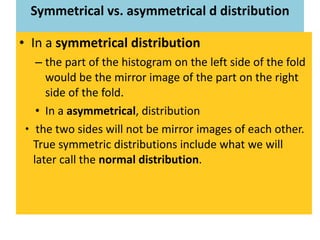
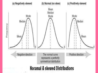
Symmetrical vs. asymmetrical d distribution In a  symmetrical distribution the part of the histogram on the left side of the fold would be the mirror image of the part on the right side of the fold.  In a  asymmetrical , distribution the two sides will not be mirror images of each other. True symmetric distributions include what we will later call the  normal distribution .
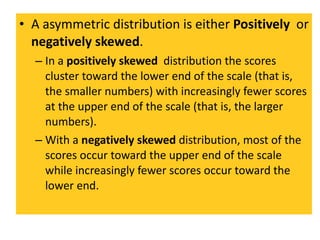
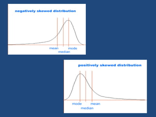
A asymmetric distribution is either  Positively  or  negatively skewed .  In a  positively skewed  distribution the scores cluster toward the lower end of the scale (that is, the smaller numbers) with increasingly fewer scores at the upper end of the scale (that is, the larger numbers). With a  negatively skewed  distribution, most of the scores occur toward the upper end of the scale while increasingly fewer scores occur toward the lower end.
 
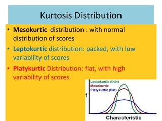
Kurtosis Distribution Mesokurtic  distribution : with normal distribution of scores Leptokurtic  distribution: packed, with low variability of scores  Platykurtic  Distribution: flat, with high variability of scores
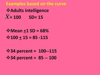
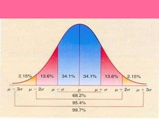
Examples based on the curve Adults intelligence  = 100  SD= 15 Mean  + 1 SD = 68% 100  +  15 = 85 -115 34 percent =  100--115  34 percent =  85 -- 100
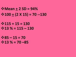
Mean  +  2 SD = 94% 100  +  (2 X 15) = 70 --130  115 + 15 = 130 13 % = 115 – 130  85 – 15 = 70 13 % = 70 –85
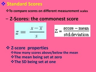
Standard Scores To compare scores on different measurement  scales Z-Scores: the commonest score  Z-score  properties How many scores above/below the mean The mean being set at zero The SD being set at one
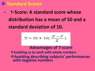
Standard Scores T -Score: A standard score whose distribution has a mean of 50 and a standard deviation of 10.   Advantages of T-score Enabling us to work with whole numbers Avoiding describing subjects’ performances  with negative numbers
 
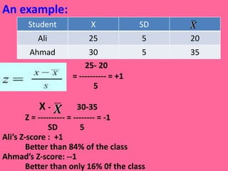
An example: _   25- 20     = ---------- = +1   5   X   -  30-35   Z = ---------- = -------- = -1 SD   5 Ali’s Z-score :  +1 Better than 84% of the class Ahmad’s Z-score: --1 Better than only 16% 0f the class Student X SD Ali 25 5 20 Ahmad 30 5 35
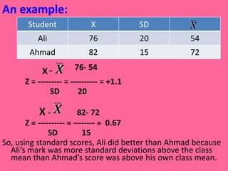
An example: _   X   –    76- 54   Z = --------- = ---------- = +1.1   SD   20   X   -  82- 72   Z = ---------- = -------- =  0.67 SD   15 So, using standard scores, Ali did better than Ahmad because Ali’s mark was more standard deviations above the class mean than Ahmad’s score was above his own class mean. Student X SD Ali 76 20 54 Ahmad 82 15 72
 
 
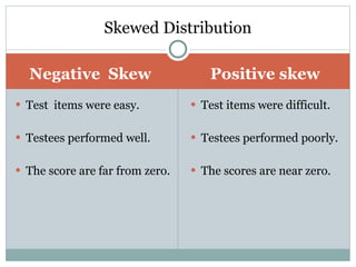
Negative  Skew Positive skew Test  items were easy. Testees performed well. The score are far from zero.  Test items were difficult. Testees performed poorly. The scores are near zero. Skewed Distribution
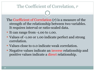
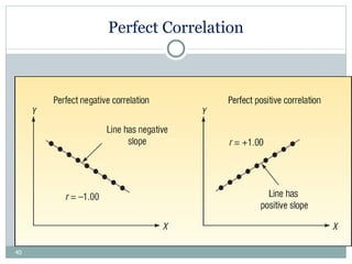
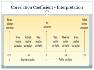
The Coefficient of Correlation,  r The  Coefficient of Correlation  ( r )  is a measure of the strength of the relationship between two variables. It requires interval or ratio-scaled data.  It can range from -1.00 to 1.00. Values of -1.00 or 1.00 indicate perfect and strong correlation. Values close to 0.0 indicate weak correlation. Negative values indicate an  inverse  relationship and positive values indicate a  direct  relationship.
Perfect Correlation
Correlation Coefficient - Interpretation
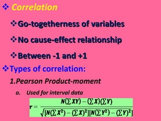
Correlation Go-togetherness of variables No cause-effect relationship Between -1 and +1 Types of correlation: Pearson Product-moment Used for interval data
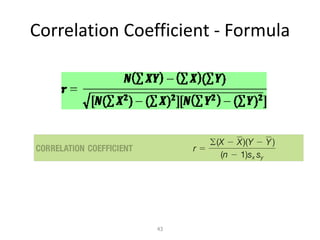
Correlation Coefficient - Formula
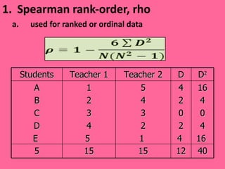
Spearman rank-order, rho used for ranked or ordinal data Students Teacher 1 Teacher 2 D D 2 A B C D E  1 2 3 4 5  5 4 3 2 1  4 2 0 2 4  16 4 0 4 16  5 15 15 12 40
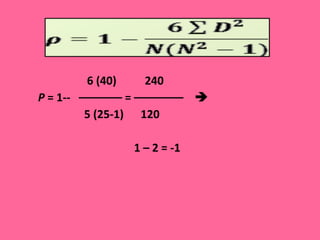
  6 (40)  240   P  = 1--  ––––––– = ––––––––     5 (25-1)  120     1 – 2 = -1
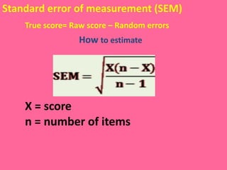
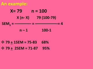
Standard error of measurement (SEM) True score= Raw score – Random errors How  to estimate  X = score n = number of items
An example: X= 79  n = 100  X (n- X)  79 (100-79)  SEM X  = –––––––– = –––––––––––= 4 n – 1  100-1 79  +  1SEM = 75-83  68% 79  +   2SEM = 71-87  95%
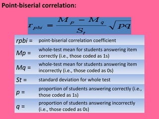
Point-biserial correlation:  rpbi  = point-biserial correlation coefficient Mp  = whole-test mean for students answering item correctly (i.e., those coded as 1s) Mq  = whole-test mean for students answering item incorrectly (i.e., those coded as 0s) St  = standard deviation for whole test p  = proportion of students answering correctly (i.e., those coded as 1s) q  = proportion of students answering incorrectly (i.e., those coded as 0s)
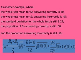
As another example, where  the whole-test mean for Ss answering correctly is 30;  the whole-test mean for Ss answering incorrectly is 45; the standard deviation for the whole test is still 8.29;  the proportion of Ss answering correctly is still .50;  and the proportion answering incorrectly is still .50 .
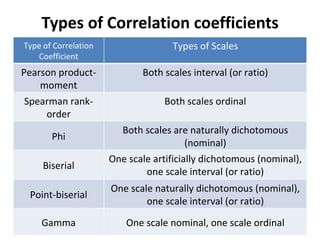
Types of Correlation coefficients Type of Correlation Coefficient Types of Scales Pearson product-moment Both scales interval (or ratio) Spearman rank-order Both scales ordinal Phi Both scales are naturally dichotomous (nominal) Biserial One scale artificially dichotomous (nominal), one scale interval (or ratio) Point-biserial One scale naturally dichotomous (nominal), one scale interval (or ratio) Gamma One scale nominal, one scale ordinal
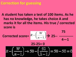
Correction for guessing A student has taken a test of 100 items. As he has no knowledge, he takes choice A and marks it for all the items. His true / corrected score is  75 Corrected score=    25--  ------------  4—1 25-25= 0
Some other factors affecting a person’s score: Practice effect Coaching effect Ceiling effect Test compromise Test Method Test Taker’s characteristics
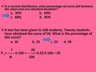
In a normal distribution, what percentage of scores fall between the mean and one standard deviation?   a.  35%  b.  50% c.  68% d.   95%  A test has been given to 100 students. Twenty students have obtained the score of 50. What is the percentage of this score? a. 10    b. 15    c. 20   d. 30  f  20 P  x = ------ X 100 = ------= 0.20 X 100 = 20 N  100
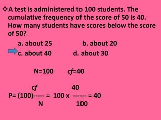
A test is administered to 100 students. The cumulative frequency of the score of 50 is 40. How many students have scores below the score of 50? a. about 25  b. about 20  c. about 40  d. about 30   N=100    cf =40 c f  40   P= (100)-----   =  100 x  ------ = 40 N  100
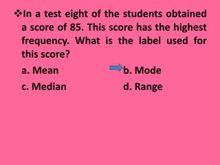
In a test eight of the students obtained a score of 85. This score has the highest frequency. What is the label used for this score? a. Mean    b. Mode  c. Median     d. Range
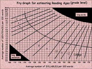
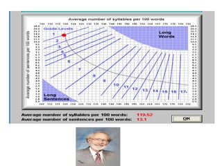
Fry’s Readability Graph Directions for Use Randomly select three 100-word passages from a book or an article. Plot the average number of syllables and the average number of sentences per 100 words on the graph to determine the grade level of the material. Choose more passages per book if great variability is observed and conclude that the book has uneven readability. Few books will fall into the solid black area, but when they do, grade level scores are invalid.
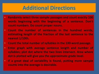
Additional Directions Randomly select three sample passages and count exactly 100 words beginning with the beginning of a sentence. Don't count numbers. Do count proper nouns. Count the number of sentences in the hundred words, estimating length of the fraction of the last sentence to the nearest 1/10th. Count the total number of syllables in the 100-word passage.  Enter graph with average sentence length and number of syllables; plot dot where the two lines intersect. Area where dot is plotted will give you the approximate grade level. If a great deal of variability is found, putting more sample counts into the average is desirable.