Salmon cycle

Salmon cycle

• 2.
  安井翔太 /  Shota  Yasui   Twitter:  @housecat442         <けーれき>   ¡  日本のド文系経済学部   アメリカで計量経済学１年   ノルウェーで資源・環境経済学修士取得   SNF研究所でデータ分析（環境税作成）   ¡  ネット広告代理店でデータ分析   ¡  ¡  ¡  §  アトリビューション分析   §  マス広告評価   動画広告評価   Etc…   §  §   
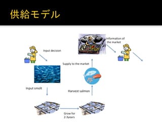
• 4.
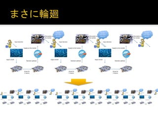
  !"2)-(,:)"&)2& &%8/&(,-9/% ;/<=>/& "/?%&="#$%& ,()$"% !"#$%&>/<='=)" !"2)-(,:)"&)2& &%8/&(,-9/% !"#$%&>/<='=)" 7$##*6&%)&%8/&(,-9/% !"#$%&'()*% !"#$%&'()*% !"#$%&>/<='=)" !"#$%&'()*% ;/<=>/& "/?%&="#$%& ,()$"% !"#$%&>/<='=)" 7$##*6&%)&%8/&(,-9/% +,-./'%&',*()"& 0-)1&2)-& 3456/,-' !"2)-(,:)"&)2& &%8/&(,-9/% ;/<=>/& "/?%&="#$%& ,()$"% !"2)-(,:)"&)2& &%8/&(,-9/% !"#$%&>/<='=)" 7$##*6&%)&%8/&(,-9/% !"#$%&'()*% +,-./'%&',*()"& 0-)1&2)-& 3456/,-' 7$##*6&%)&%8/&(,-9/% !"#$%&'()*% +,-./'%&',*()"& 0-)1&2)-& 3456/,-' !"2)-(,:)"&)2& &%8/&(,-9/% !"#$%&'()*% +,-./'%&',*()"& 0-)1&2)-& 3456/,-' !"2)-(,:)"&)2& &%8/&(,-9/% ;/<=>/& "/?%&="#$%& ,()$"% !"#$%&>/<='=)" 7$##*6&%)&%8/&(,-9/% !"#$%&'()*% 0-)1&2)-& 3456/,-' ;/<=>/& "/?%&="#$%& ,()$"% !"#$%&>/<='=)" 7$##*6&%)&%8/&(,-9/% +,-./'%&',*()"& 0-)1&2)-& 3456/,-' ;/<=>/& "/?%&="#$%& ,()$"% !"#$%&>/<='=)" +,-./'%&',*()"& 0-)1&2)-& 3456/,-' ;/<=>/& "/?%&="#$%& ,()$"% !"2)-(,:)"&)2& &%8/&(,-9/% 7$##*6&%)&%8/&(,-9/% +,-./'%&',*()"& !"2)-(,:)"&)2& &%8/&(,-9/% ;/<=>/& "/?%&="#$%& ,()$"% ;/<=>/& "/?%&="#$%& ,()$"% !"#$%&>/<='=)" 7$##*6&%)&%8/&(,-9/% !"#$%&'()*% !"2)-(,:)"&)2& &%8/&(,-9/% +,-./'%&',*()"& 0-)1&2)-& 3456/,-' ;/<=>/& "/?%&="#$%& ,()$"% !"#$%&>/<='=)" 7$##*6&%)&%8/&(,-9/% !"#$%&'()*% !"2)-(,:)"&)2& &%8/&(,-9/% +,-./'%&',*()"& 0-)1&2)-& 3456/,-' ;/<=>/& "/?%&="#$%& ,()$"% !"#$%&>/<='=)" 7$##*6&%)&%8/&(,-9/% !"#$%&'()*% !"2)-(,:)"&)2& &%8/&(,-9/% +,-./'%&',*()"& 0-)1&2)-& 3456/,-' !"#$%&>/<='=)" 7$##*6&%)&%8/&(,-9/% !"#$%&'()*% !"2)-(,:)"&)2& &%8/&(,-9/% +,-./'%&',*()"& 0-)1&2)-& 3456/,-' 7$##*6&%)&%8/&(,-9/% !"#$%&'()*% +,-./'%&',*()"& 0-)1&2)-& 3456/,-' ;/<=>/ "/?%&="# ,()$"
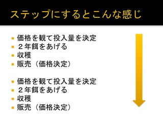
• 5.
  ¡  価格を観て投入量を決定   ¡ ２年餌をあげる   ¡  収穫   ¡  販売（価格決定）   ¡  価格を観て投入量を決定   ¡  ２年餌をあげる   ¡  収穫   ¡  販売（価格決定）  
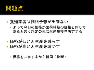
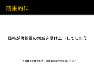
• 6.
  ¡  養殖業者は価格予想が出来ない   § よって今日の価格が出荷時期の価格と同じで あると言う想定の元に生産規模を決定する   ¡  価格が低いと生産を減らす   ¡  価格が高いと生産を増やす   §  価格を共有するから皆同じ決断！  
• 7.
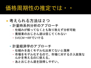
  価格が供給量の増減を受け上下してしまう この構造を推定して、価格の周期性を説明したい！
• 8.
  ¡  考えられる方法は２つ   § 計量時系列分析のアプローチ   ▪  仕組みが解ってなくとも取り敢えず分析可能   ▪  養殖業のおじさん達は信じてくれない   ▪  SVECM→IRFでいける   §  計量経済学のアプローチ   ▪  仕組みを良くモデル化出来てないと藻屑   ▪  市場をモデル化するので、市場に対する介入政策な んかを考えるのに使える。   ▪  あとおじさん達を説得しやすい。
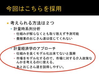
• 9.
  ¡  考えられる方法は２つ   § 計量時系列分析   ▪  仕組みが解らなくとも取り敢えず予測可能   ▪  養殖業のおじさん達は信じてくれない   §  計量経済学のアプローチ   ▪  仕組みを良くモデル化出来てないと藻屑   ▪  市場をモデル化するので、市場に対する介入政策な んかを考えるのに使える。   ▪  あとおじさん達を説得しやすい。
• 10.
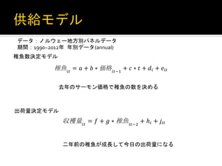
  データ：ノルウェー地方別パネルデータ   期間：1990~2012年 年別データ(annual)   稚魚数決定モデル !" =!+!∗ !"!! + ! ∗ ! + !! + !!" 去年のサーモン価格で稚魚の数を決める 出荷量決定モデル !" =!+!∗ !"!! + ℎ! + !!" 二年前の稚魚が成長して今日の出荷量になる
• 11.
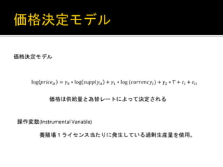
  two years before.Basically this equation describes that how many percentage of salmon is going to be produced when the smolt input is increased by 1%. Combining these above two equations, it is possible to see the effect of the price of farmed salmon in year t-3 on the supply quantity in year t. 価格決定モデル Equation3: Demand equation (price determination) model log !"#$!!" = !! ∗ log !"##$!!" + !! ∗ log!(!"##$%!!! ) + !! ∗ ! + !! + !!" 価格は供給量と為替レートによって決定される Demand equation (equation3) has price of farmed salmon as the dependent variable. Explanatory variable 操作変数(Instrumental  Variable)   is supply quantity, currency rate and time trend.   Since  養殖場１ライセンス当たりに発生している過剰生産量を使用。 the price is determined by total supply in the market, the total supply amount is used in here instead of supply per license. Currency rate is the real rate between France and Norway. Because France is the biggest importer of Norwegian Farmed
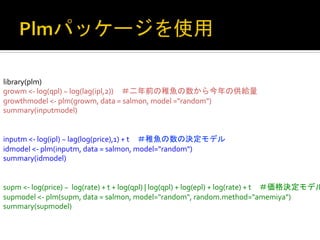
• 12.
  library(plm)   growm  <-­‐  log(qpl)  ~  log(lag(ipl,2))　＃二年前の稚魚の数から今年の供給量   growthmodel  <-­‐  plm(growm,  data  =  salmon,  model  ="random")   summary(inputmodel)       inputm  <-­‐  log(ipl)  ~  lag(log(price),1)  +  t　＃稚魚の数の決定モデル   idmodel  <-­‐  plm(inputm,  data  =  salmon,  model="random")   summary(idmodel)       supm  <-­‐  log(price)  ~    log(rate)  +  t  +  log(qpl)  |  log(qpl)  +  log(epl)  +  log(rate)  +  t　＃価格決定モデル supmodel  <-­‐  plm(supm,  data  =  salmon,  model="random",  random.method="amemiya")   summary(supmodel)
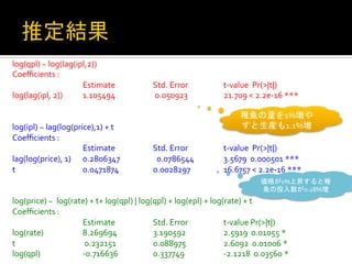
• 13.
  log(qpl)  ~  log(lag(ipl,2))   Coefficients  :                                        Estimate      Std.  Error    t-­‐value    Pr(>|t|)           log(lag(ipl,  2))    1.105494        0.050923      21.709  <  2.2e-­‐16  ***     稚魚の量を1%増や   すと生産も1.1%増 log(ipl)  ~  lag(log(price),1)  +  t   Coefficients  :                                            Estimate      Std.  Error    t-­‐value    Pr(>|t|)           lag(log(price),  1)    0.2806347      0.0786544      3.5679    0.000501  ***   t                                      0.0471874      0.0028297    16.6757  <  2.2e-­‐16  ***     価格が1%上昇すると稚 魚の投入数が0.28%増   log(price)  ~    log(rate)  +  t+  log(qpl)  |  log(qpl)  +  log(epl)  +  log(rate)  +  t   Coefficients  :                            Estimate      Std.  Error    t-­‐value  Pr(>|t|)       log(rate)      8.269694        3.190592      2.5919    0.01055  *   t                        0.232151        0.088975      2.6092    0.01006  *   log(qpl)        -­‐0.716636        0.337749      -­‐2.1218    0.03560  *  
• 14.
  ¡  仮定していた構造による周期性あるの？   § 推定結果的にはYes   §  でも、その影響の大きさはちゃんと検証が必要   §  やっぱりVARモデル？