RNN, Seq2Seq Learning
and Image Captioning
Dongang Wang
07 July 2017
Contents
• From RNN to LSTM
• Backpropagation through time (BPTT)
• Usage of LSTM
• Seq2Seq Learning
• Attention Mechanism
• Image Captioning
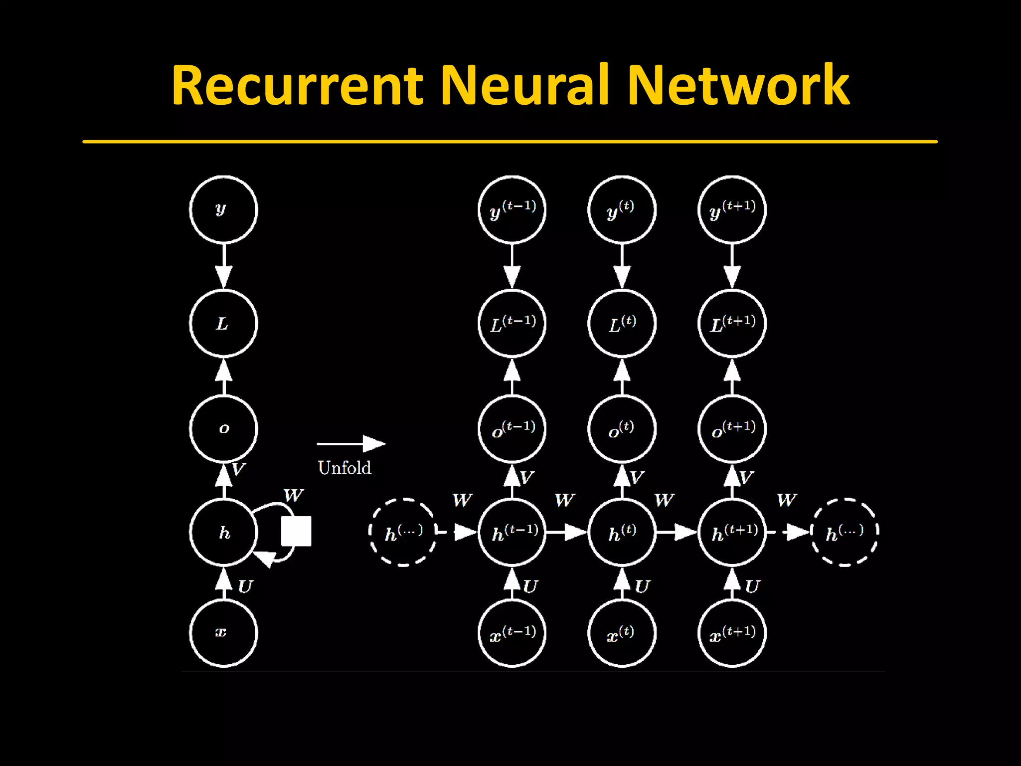
Recurrent Neural Network
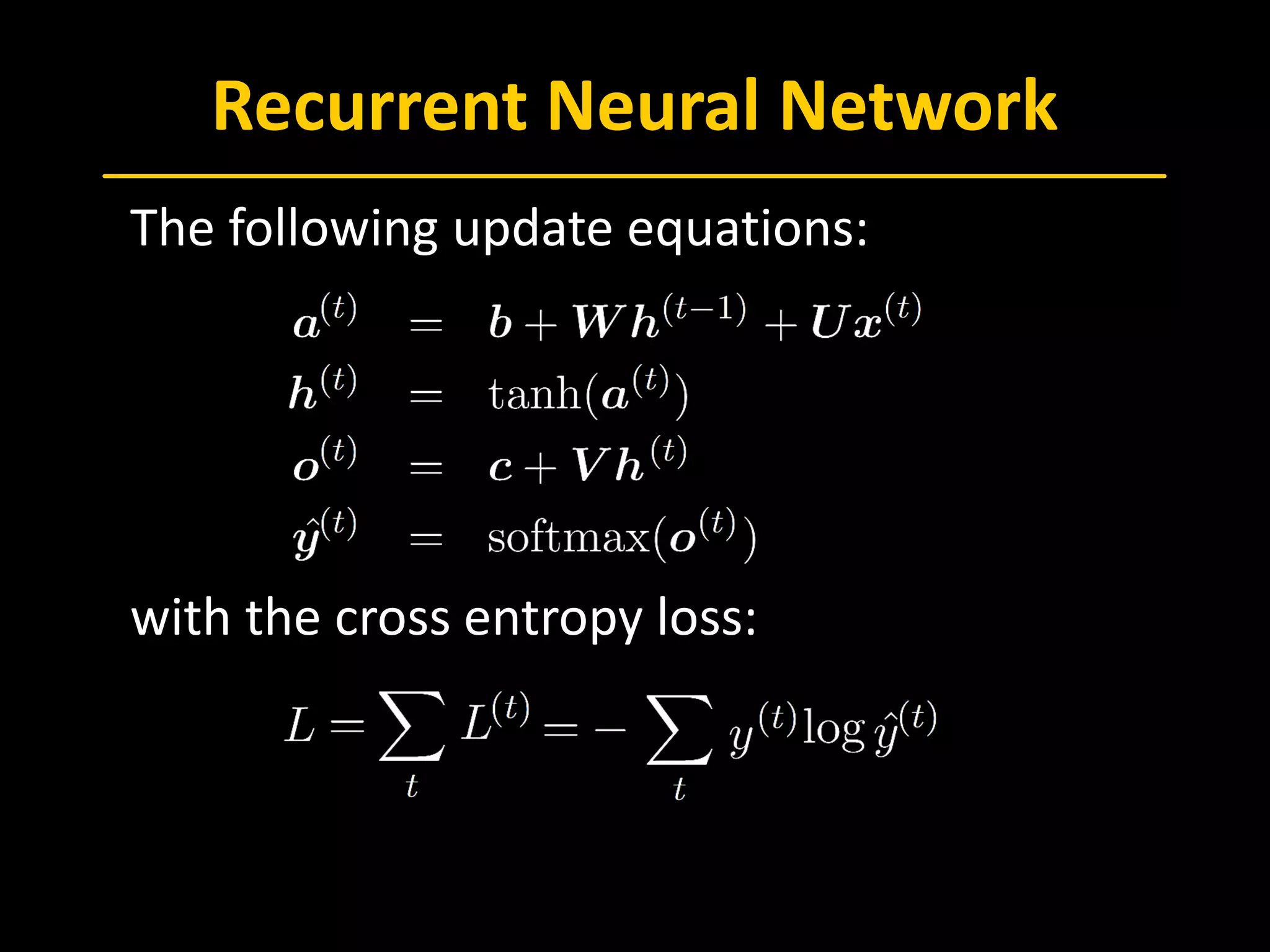
 The following update equations:
 with the cross entropy loss:
Backpropagation Through Time
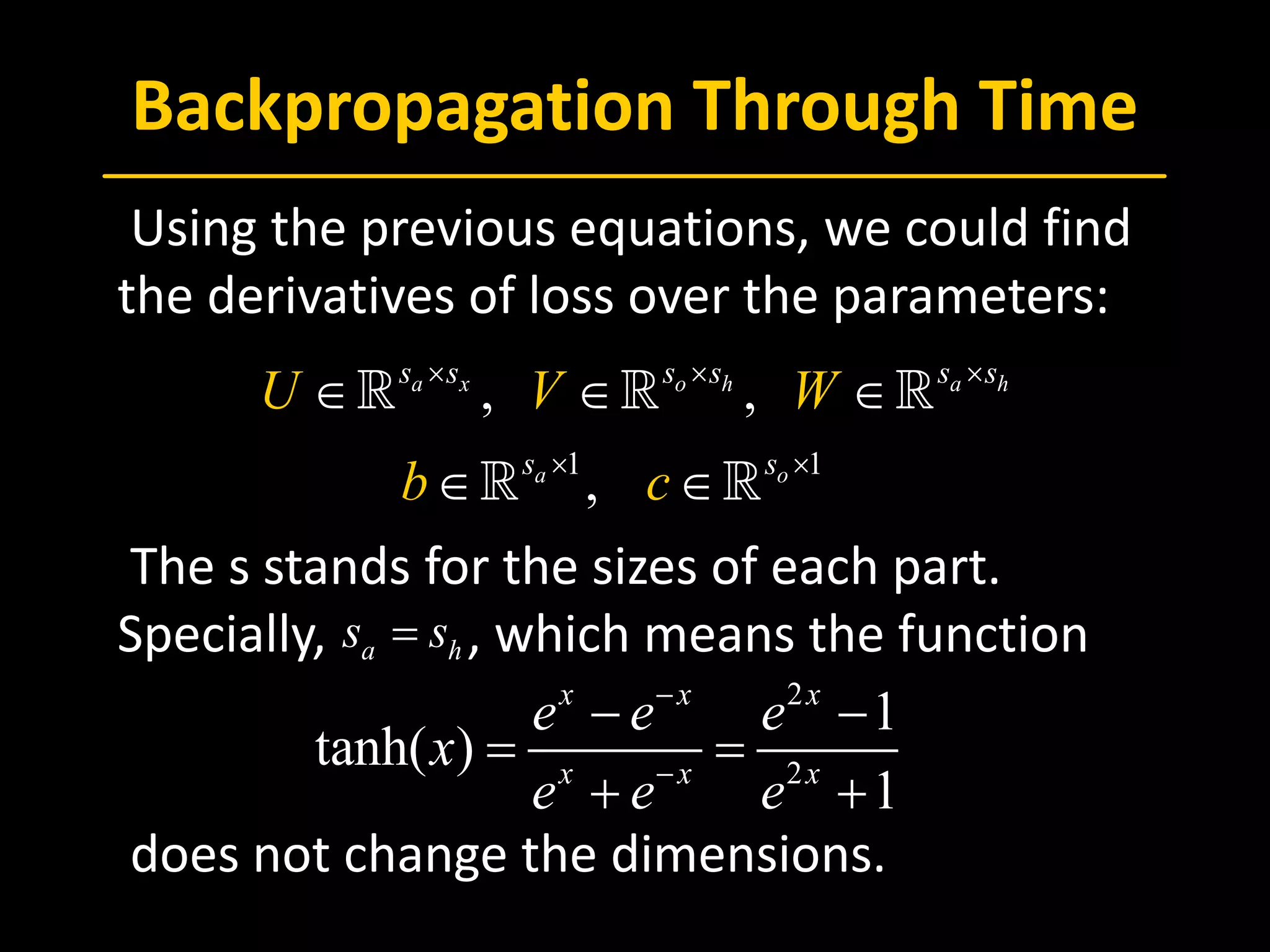
 Using the previous equations, we could find
the derivatives of loss over the parameters:
 The s stands for the sizes of each part.
Specially, , which means the function
 does not change the dimensions.
1 1
, ,
,
a x o h a h
a o
s s s s s s
s s
U V W
b c
× × ×
× ×
∈ ∈ ∈
∈ ∈
  
 
2
2
1
tanh( )
1
x x x
x x x
e e e
x
e e e
−
−
− −
= =
+ +
a hs s=
Backpropagation Through Time
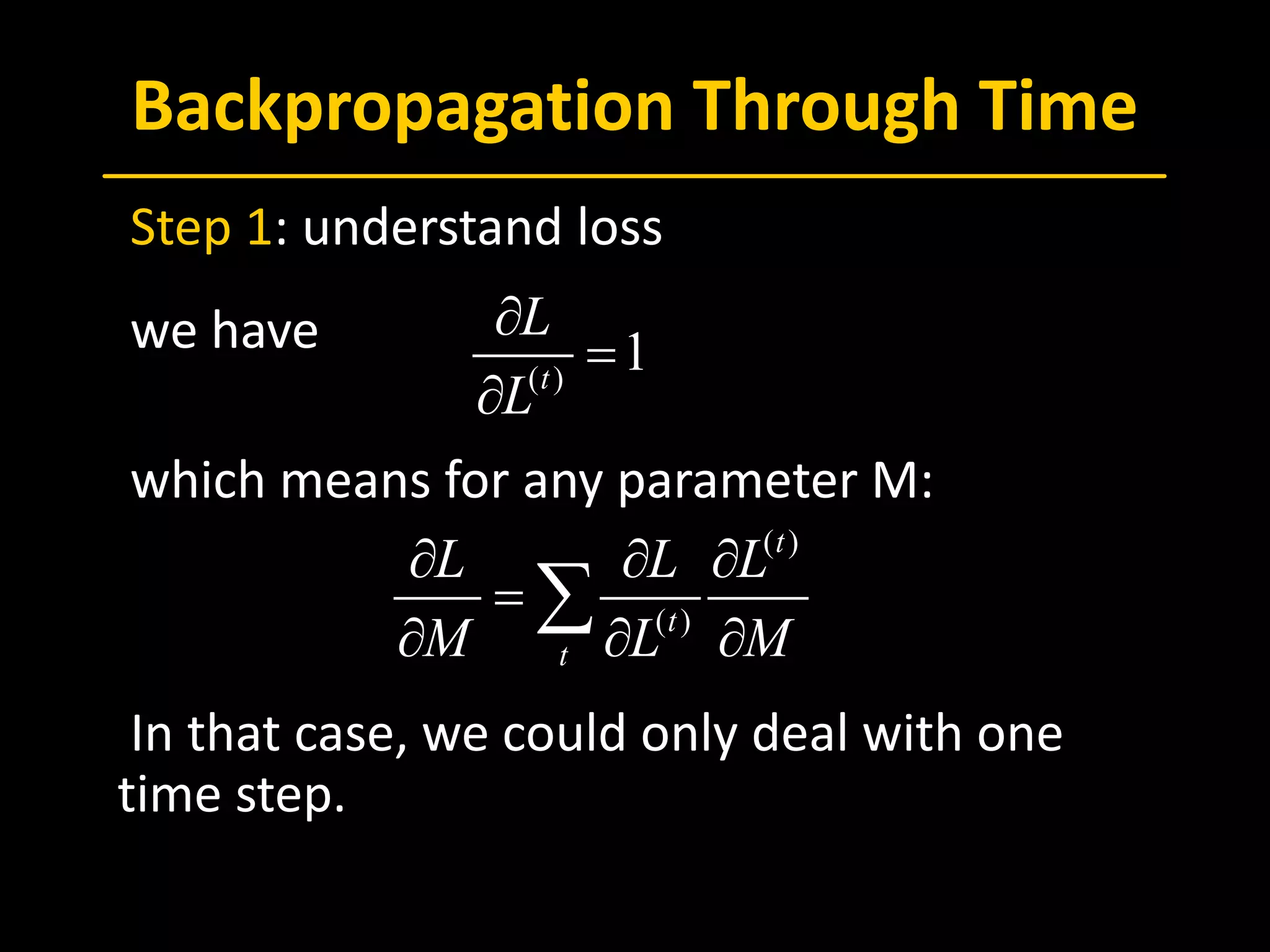
 Step 1: understand loss
 we have
 which means for any parameter M:
 In that case, we could only deal with one
time step.
, ,a x a x a xs s s s s s
U U U× × ×
∈ ∈ ∈  
( )
1t
L
L
∂
=
∂
( )
( )
t
t
t
L L L
M L M
∂ ∂ ∂
=
∂ ∂ ∂
∑
Backpropagation Through Time
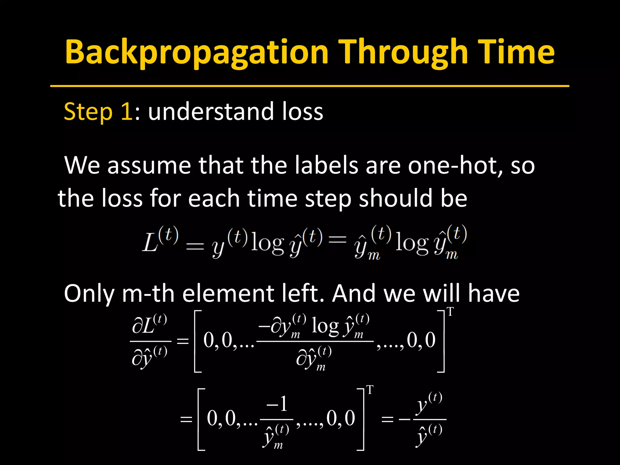
 Step 1: understand loss
 We assume that the labels are one-hot, so
the loss for each time step should be
 Only m-th element left. And we will have
T( ) ( )( )
( ) ( )
T
( )
( ) ( )
ˆlog
0,0,... ,...,0,0
ˆ ˆ
1
0,0,... ,...,0,0
ˆ ˆ
t tt
m m
t t
m
t
t t
m
y yL
y y
y
y y
 −∂∂
=  
∂ ∂ 
 −
= = − 
 
Backpropagation Through Time
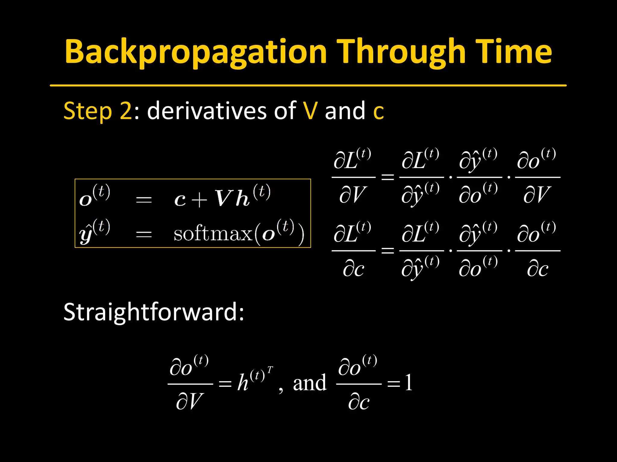
 Step 2: derivatives of V and c
 Straightforward:
( ) ( ) ( ) ( )
( ) ( )
( ) ( ) ( ) ( )
( ) ( )
ˆ
ˆ
ˆ
ˆ
t t t t
t t
t t t t
t t
L L y o
V y o V
L L y o
c y o c
∂ ∂ ∂ ∂
= ⋅ ⋅
∂ ∂ ∂ ∂
∂ ∂ ∂ ∂
= ⋅ ⋅
∂ ∂ ∂ ∂
( ) ( )
( )
, and 1
T
t t
to o
h
V c
∂ ∂
= =
∂ ∂
Backpropagation Through Time
 Step 2: derivatives of V and c
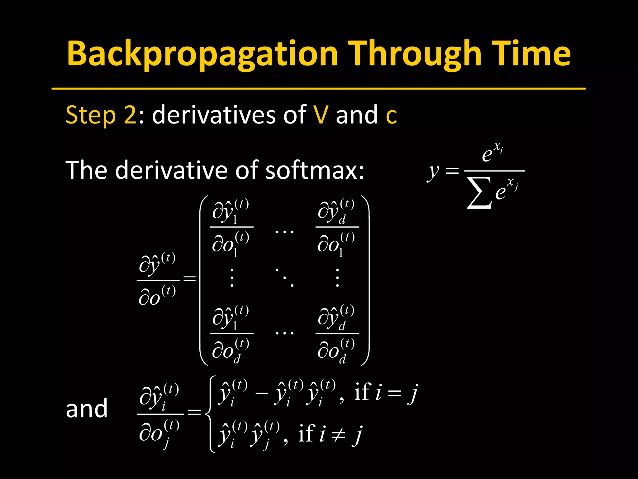
 The derivative of softmax:
 and
i
j
x
x
e
y
e
=
∑( )( )
1
( ) ( )
1 1( )
( )
( )( )
1
( ) ( )
ˆˆ
ˆ
=
ˆˆ
tt
d
t t
t
t
tt
d
t t
d d
yy
o o
y
o
yy
o o
 ∂∂
 
∂ ∂ 
∂  
 ∂
∂∂ 
 ∂ ∂ 

  

( ) ( ) ( )( )
( ) ( ) ( )
ˆ ˆ ˆ , ifˆ
=
ˆ ˆ , if
t t tt
i i ii
t t t
j i j
y y y i jy
o y y i j
 − =∂ 

∂ ≠
Backpropagation Through Time
 Step 2: derivatives of V and c
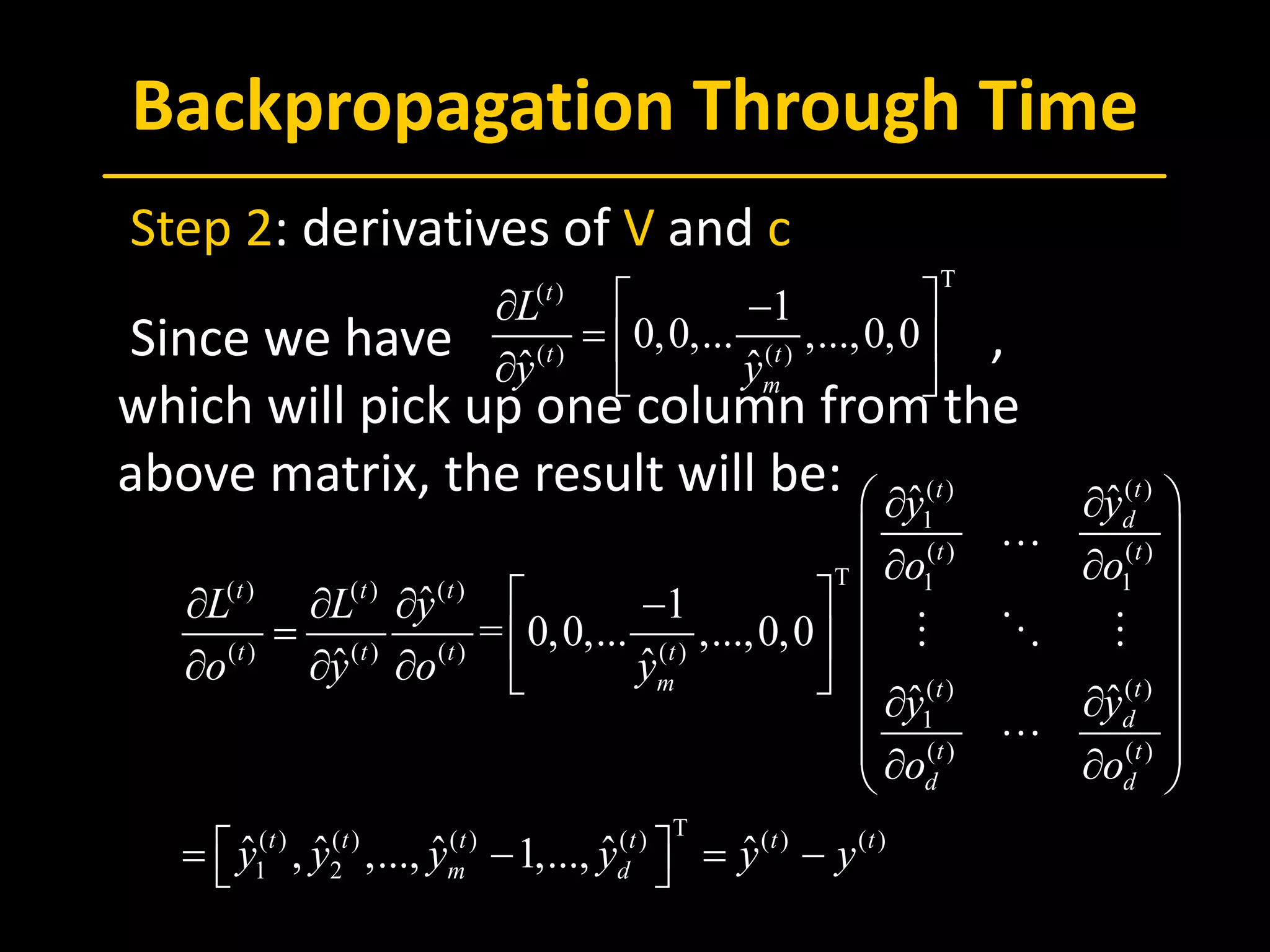
 Since we have ,
which will pick up one column from the
above matrix, the result will be:
T
( )
( ) ( )
1
0,0,... ,...,0,0
ˆ ˆ
t
t t
m
L
y y
 ∂ −
=  
∂  
( )( )
1
( ) ( )
T 1 1( ) ( ) ( )
( ) ( ) ( ) ( )
( )( )
1
( ) ( )
T( ) ( ) ( ) ( ) ( ) ( )
1 2
ˆˆ
ˆ 1
= 0,0,... ,...,0,0
ˆ ˆ
ˆˆ
ˆ ˆ ˆ ˆ ˆ, ,..., 1,...,
tt
d
t t
t t t
t t t t
m tt
d
t t
d d
t t t t t t
m d
yy
o o
L L y
o y o y
yy
o o
y y y y y y
 ∂∂
 
∂ ∂  ∂ ∂ ∂ −  =  
 ∂ ∂ ∂  
∂∂ 
 ∂ ∂ 
 = − =− 

  

Backpropagation Through Time
 Step 2: derivatives of V and c
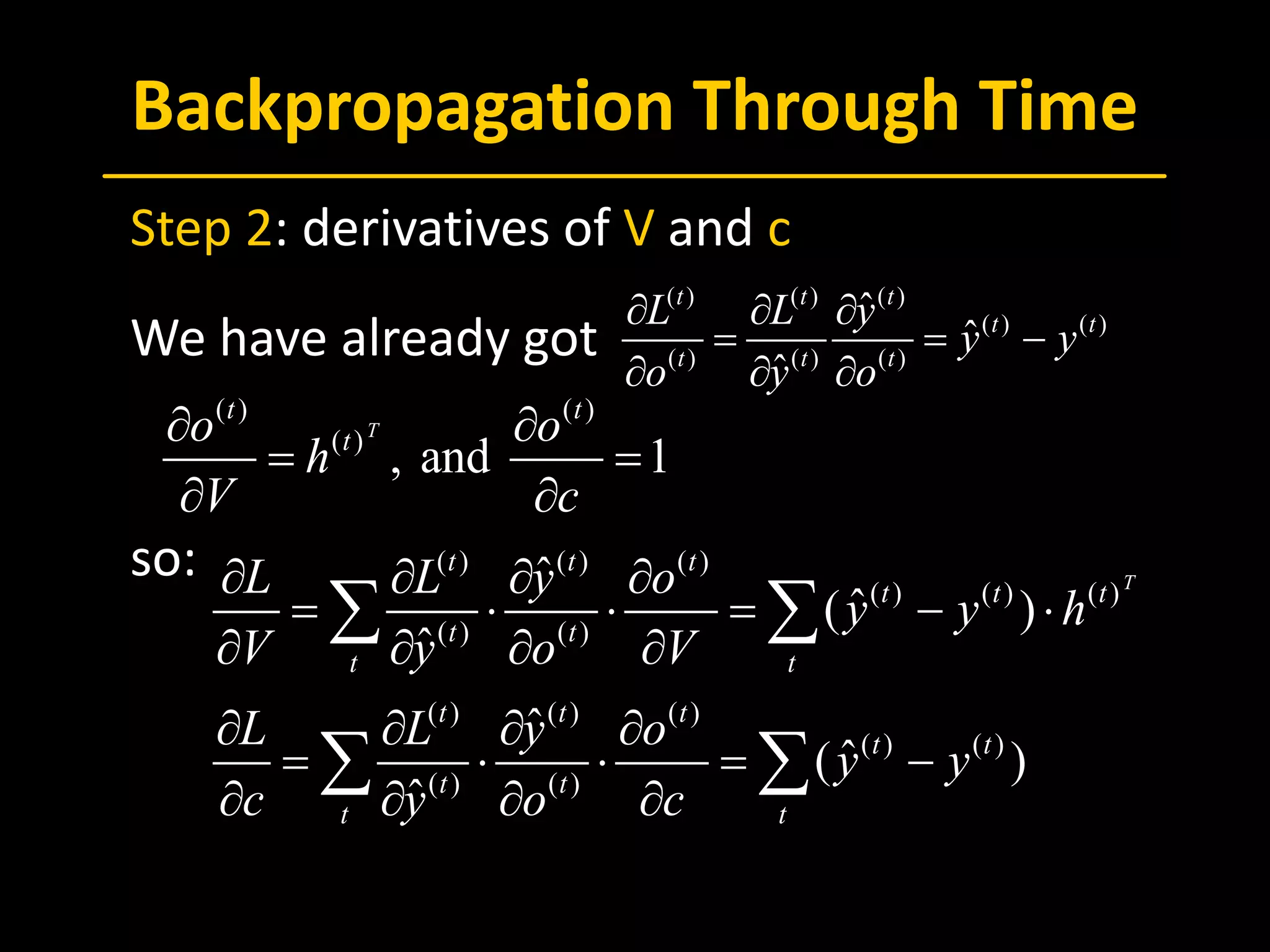
 We have already got
 
 so: ( ) ( ) ( )
( ) ( ) ( )
( ) ( )
( ) ( ) ( )
( ) ( )
( ) ( )
ˆ
ˆ( )
ˆ
ˆ
ˆ( )
ˆ
T
t t t
t t t
t t
t t
t t t
t t
t t
t t
L L y o
y y h
V y o V
L L y o
y y
c y o c
∂ ∂ ∂ ∂
= ⋅ ⋅ = − ⋅
∂ ∂ ∂ ∂
∂ ∂ ∂ ∂
= ⋅ ⋅ = −
∂ ∂ ∂ ∂
∑ ∑
∑ ∑
( ) ( )
( )
, and 1
T
t t
to o
h
V c
∂ ∂
=
∂ ∂
( ) ( ) ( )
( ) ( )
( ) ( ) ( )
ˆ
ˆ
ˆ
t t t
t t
t t t
L L y
y y
o y o
∂ ∂ ∂
= = −
∂ ∂ ∂
Backpropagation Through Time
 Step 3: derivatives of h
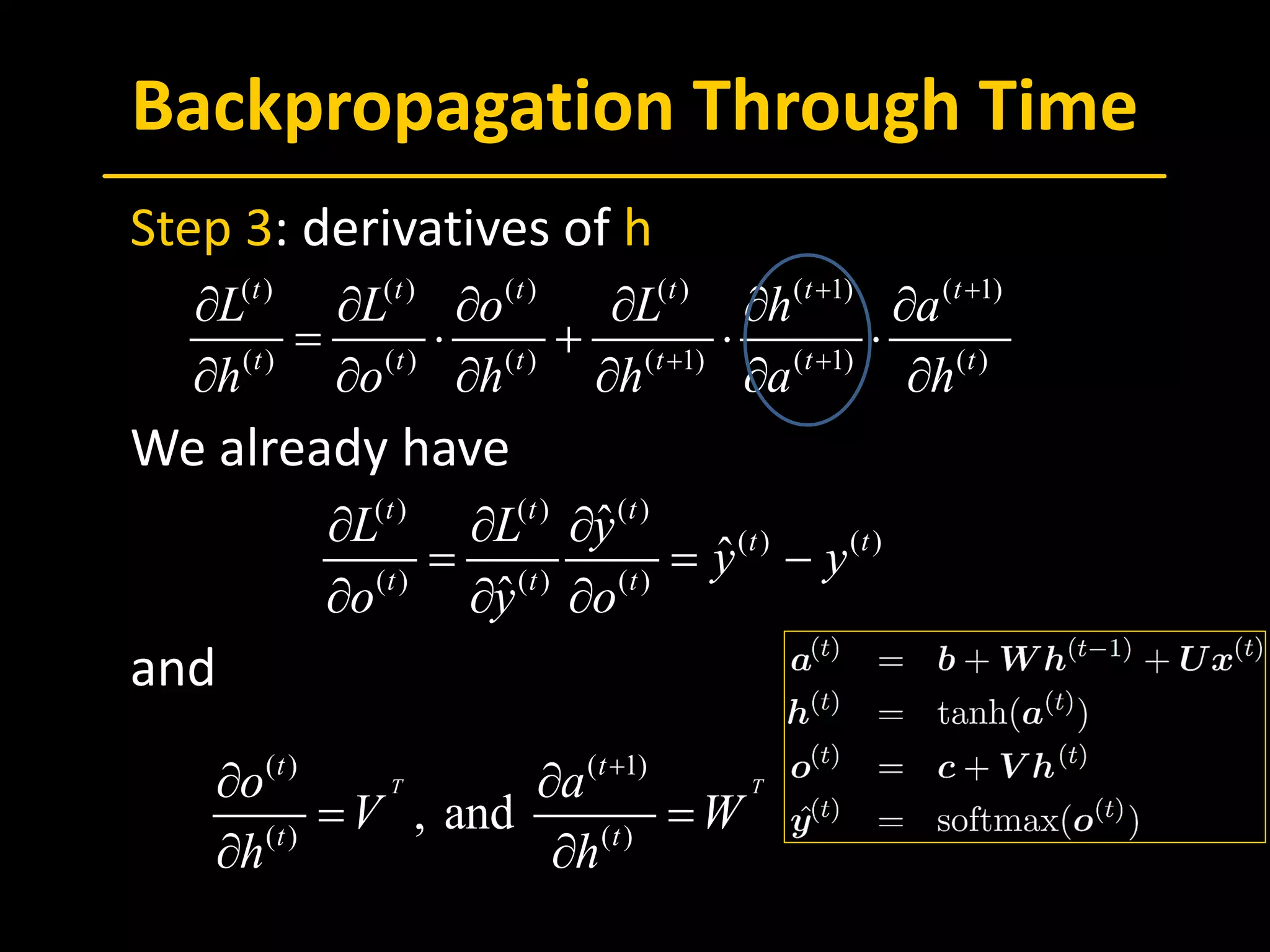
 We already have
 and
( ) ( ) ( ) ( ) ( 1) ( 1)
( ) ( ) ( ) ( 1) ( 1) ( )
t t t t t t
t t t t t t
L L o L h a
h o h h a h
+ +
+ +
∂ ∂ ∂ ∂ ∂ ∂
= ⋅ + ⋅ ⋅
∂ ∂ ∂ ∂ ∂ ∂
( ) ( ) ( )
( ) ( )
( ) ( ) ( )
ˆ
ˆ
ˆ
t t t
t t
t t t
L L y
y y
o y o
∂ ∂ ∂
= = −
∂ ∂ ∂
( ) ( 1)
( ) ( )
, and
T T
t t
t t
o a
V W
h h
+
∂ ∂
= =
∂ ∂
Backpropagation Through Time
 Step 3: derivatives of h
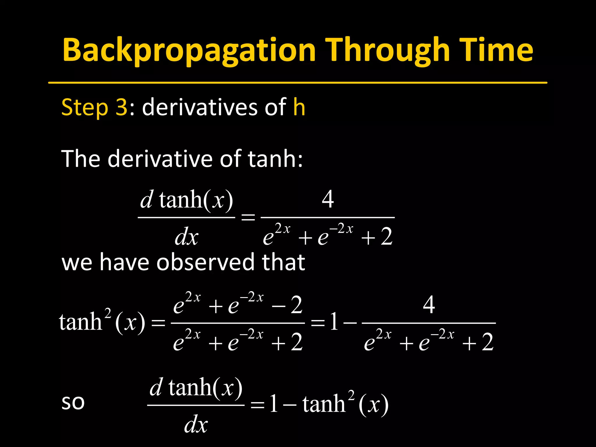
 The derivative of tanh:
 we have observed that
 so
2 2
tanh( ) 4
2x x
d x
dx e e−
=
+ +
2 2
2
2 2 2 2
2 4
tanh ( ) 1
2 2
x x
x x x x
e e
x
e e e e
−
− −
+ −
= = −
+ + + +
2tanh( )
1 tanh ( )
d x
x
dx
= −
Backpropagation Through Time
 Step 3: derivatives of h
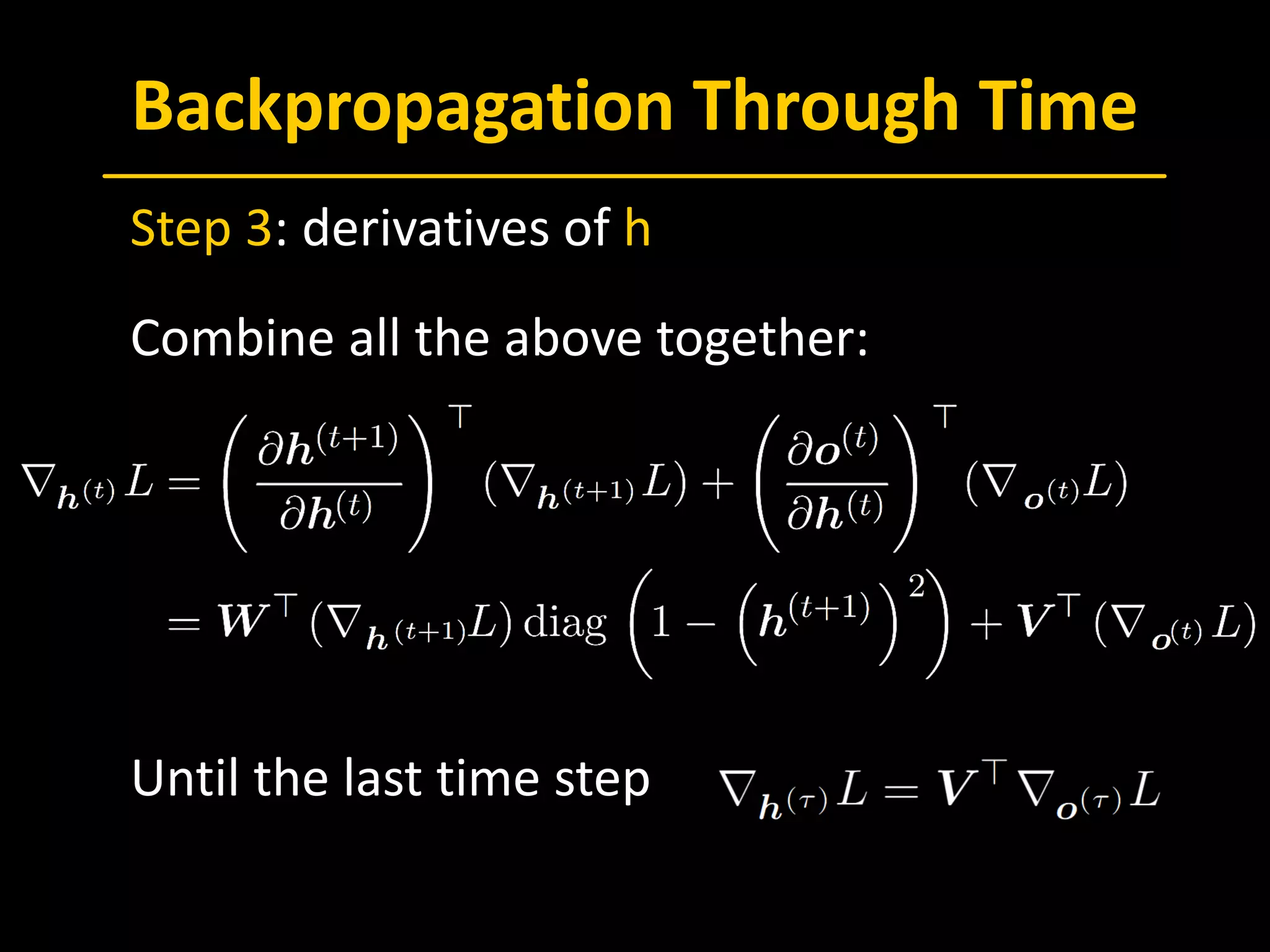
 Combine all the above together:
 Until the last time step
Backpropagation Through Time
 Step 4: derivatives of U, W and b
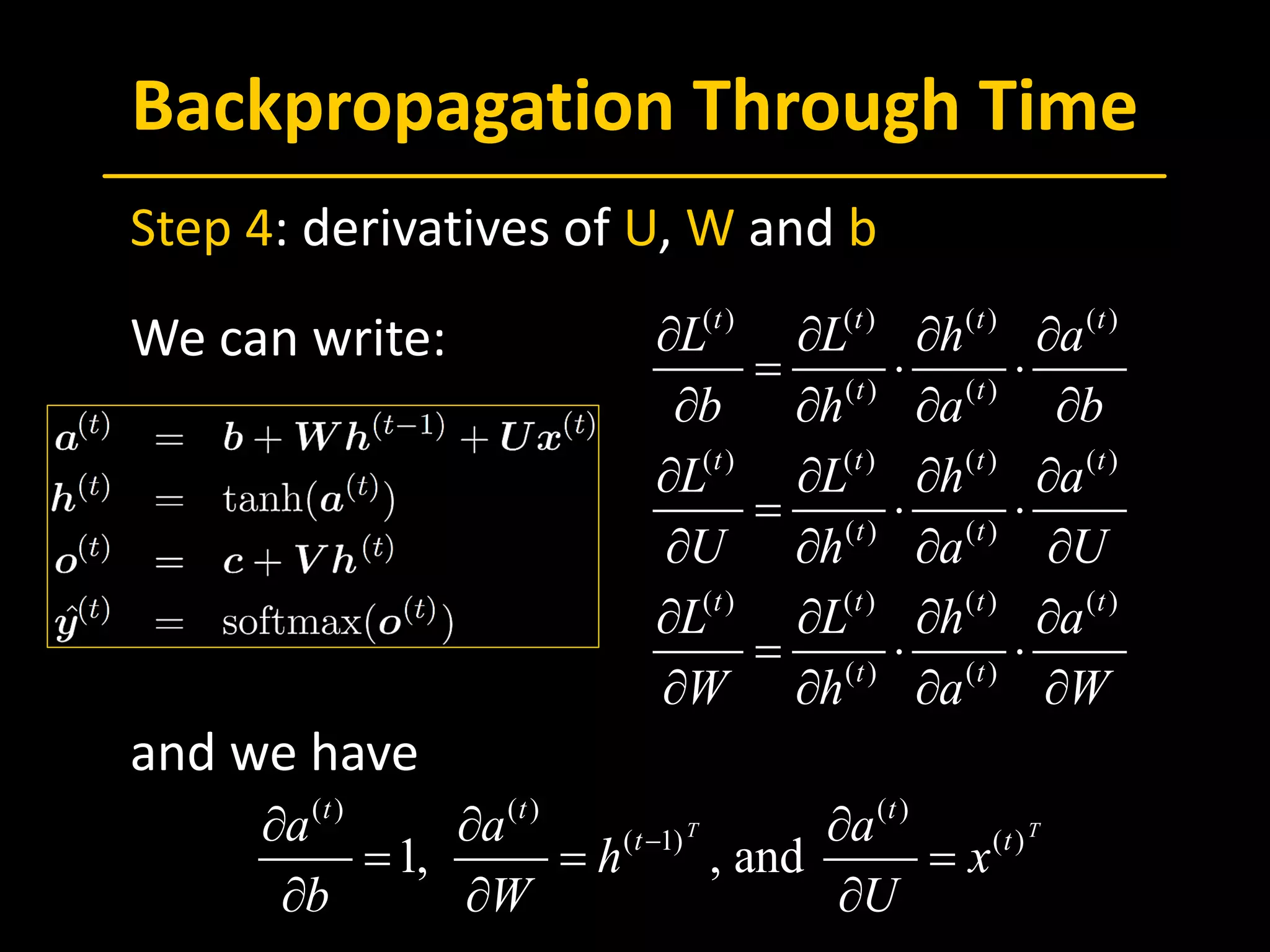
 We can write:
 and we have
( ) ( ) ( ) ( )
( ) ( )
( ) ( ) ( ) ( )
( ) ( )
( ) ( ) ( ) ( )
( ) ( )
t t t t
t t
t t t t
t t
t t t t
t t
L L h a
b h a b
L L h a
U h a U
L L h a
W h a W
∂ ∂ ∂ ∂
= ⋅ ⋅
∂ ∂ ∂ ∂
∂ ∂ ∂ ∂
= ⋅ ⋅
∂ ∂ ∂ ∂
∂ ∂ ∂ ∂
= ⋅ ⋅
∂ ∂ ∂ ∂
( ) ( ) ( )
( 1) ( )
1, , and
T T
t t t
t ta a a
h x
b W U
−∂ ∂ ∂
= = =
∂ ∂ ∂
Backpropagation Through Time
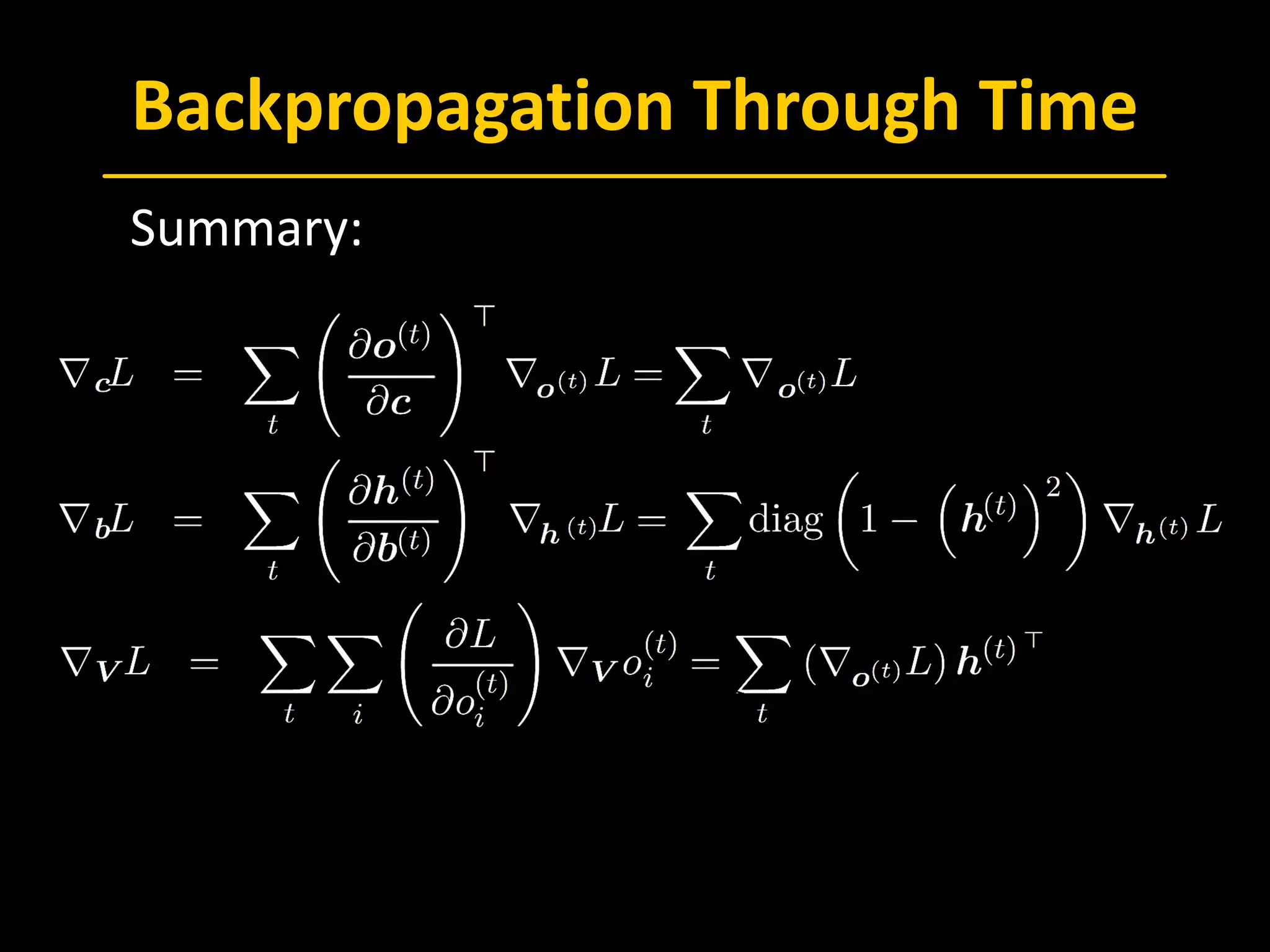
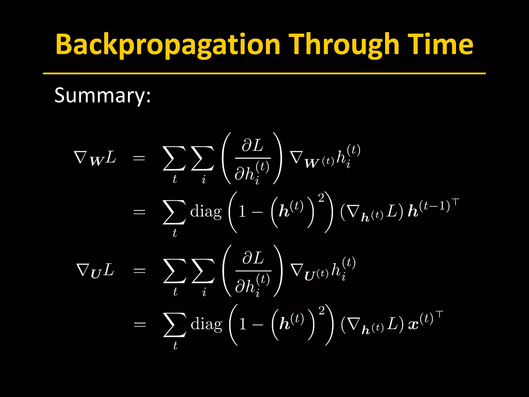
 Summary:
Backpropagation Through Time
 Summary:
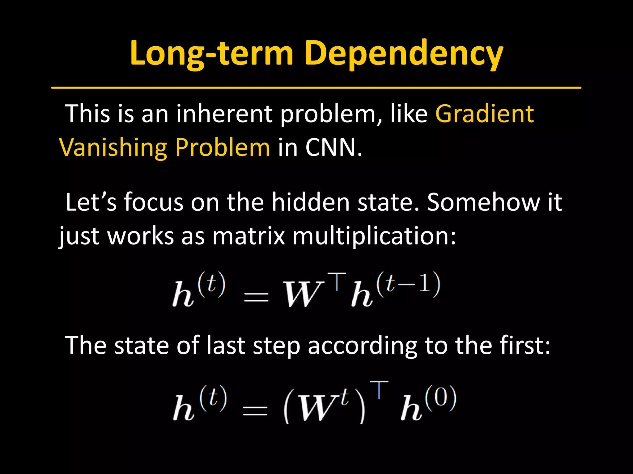
Long-term Dependency
 This is an inherent problem, like Gradient
Vanishing Problem in CNN.
 Let’s focus on the hidden state. Somehow it
just works as matrix multiplication:
 The state of last step according to the first:
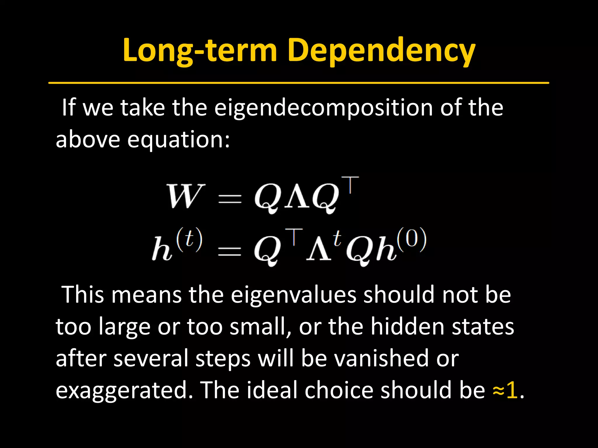
Long-term Dependency
 If we take the eigendecomposition of the
above equation:
 This means the eigenvalues should not be
too large or too small, or the hidden states
after several steps will be vanished or
exaggerated. The ideal choice should be ≈1.
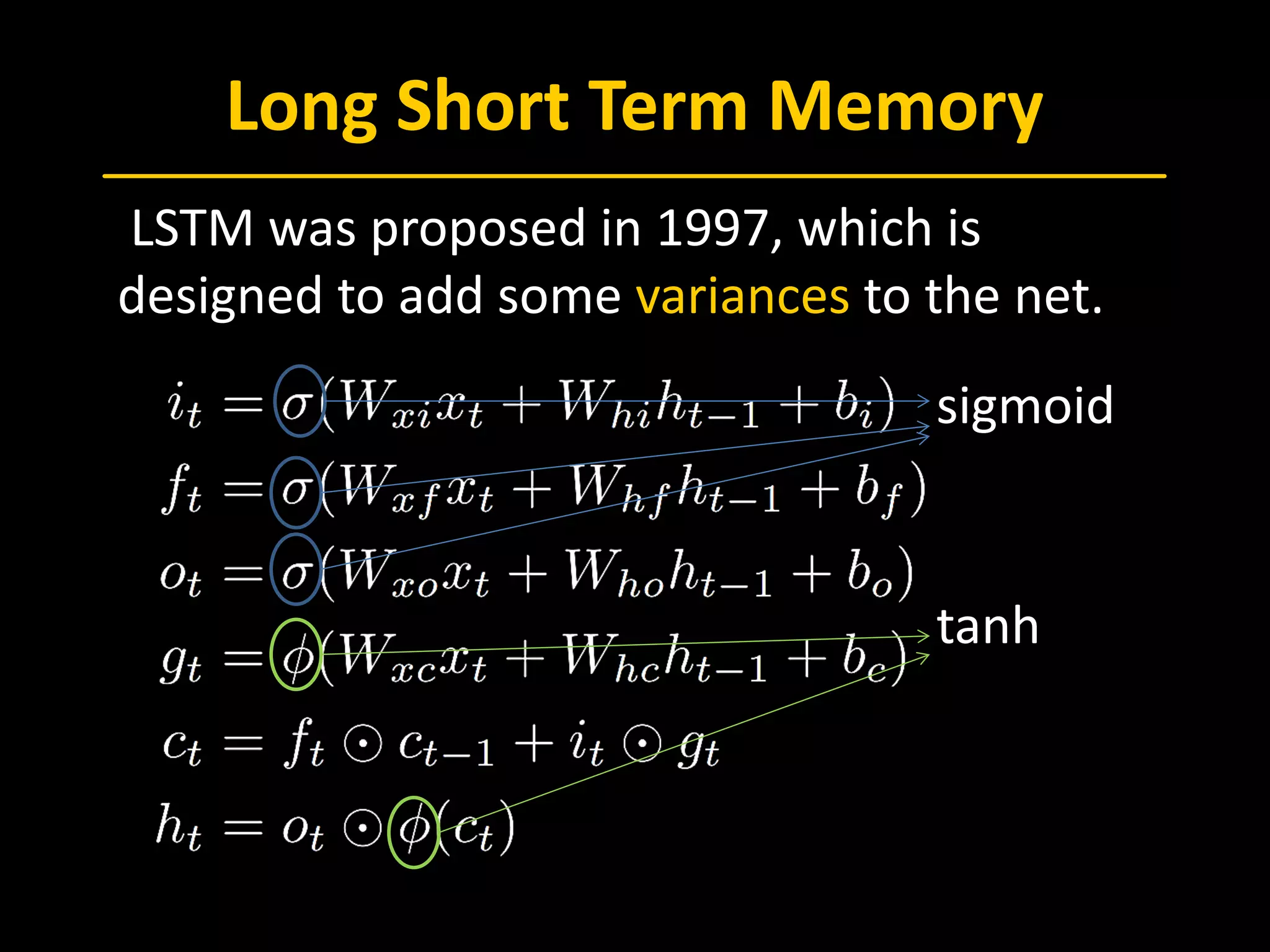
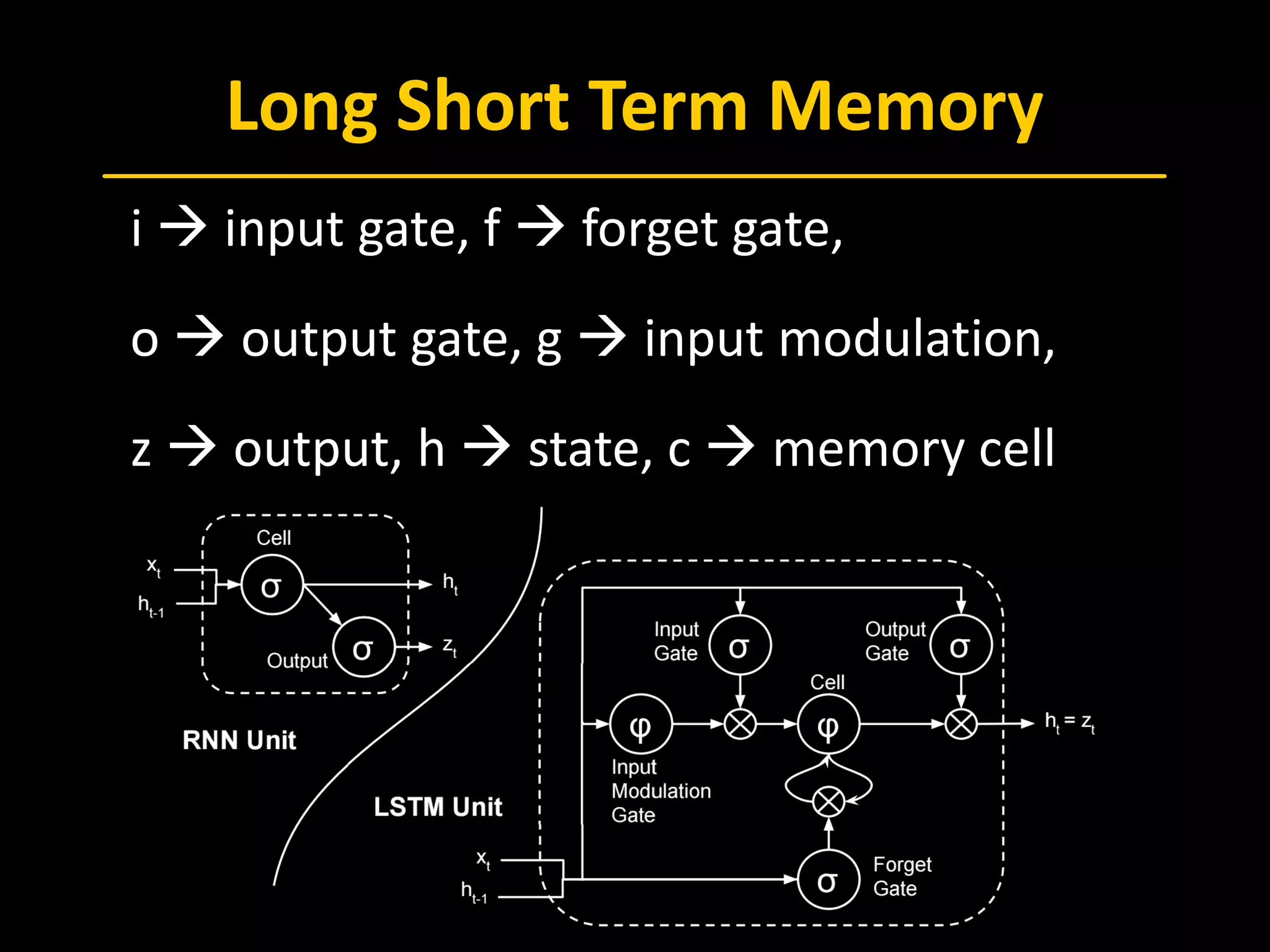
Long Short Term Memory
 LSTM was proposed in 1997, which is
designed to add some variances to the net.
  sigmoid
  tanh
Long Short Term Memory
 i  input gate, f  forget gate,
 o  output gate, g  input modulation,
 z  output, h  state, c  memory cell
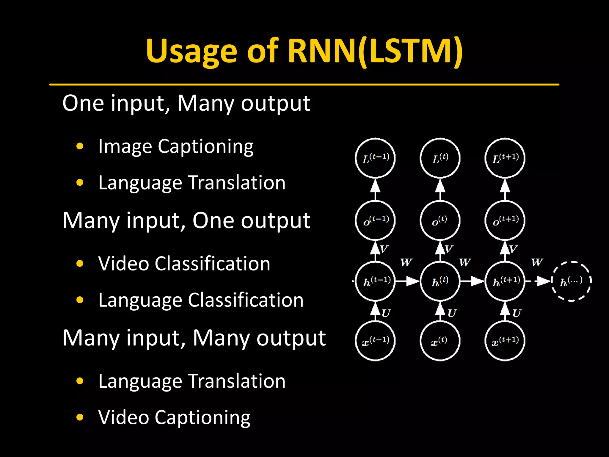
Usage of RNN(LSTM)
 One input, Many output
• Image Captioning
• Language Translation
 Many input, One output
• Video Classification
• Language Classification
 Many input, Many output
• Language Translation
• Video Captioning
Seq2Seq
 One successful implementation of LSTM is
Sequence-to-Sequence learning. This is first
introduced to solve machine translation
problems (kind of transfer learning).
– Sequence to sequence learning with neural
networks (2014)
– Learning Phrase Representation using RNN
Encoder-Decoder for Statistical Machine
Translation (2014)
Seq2Seq
 NLP fundations:
• word embedding
There are two ways to represent word. One is using
dictionary, and each word will be a one-hot vector. The
other way is using word embedding tools like
word2vec.
• beam searching
For output, each time there will be an output of
softmax probabilities. It is not fair to choose the word
with largest prob as the prediction. Instead, we choose
k largest each time, where k is the beam size.
Seq2Seq
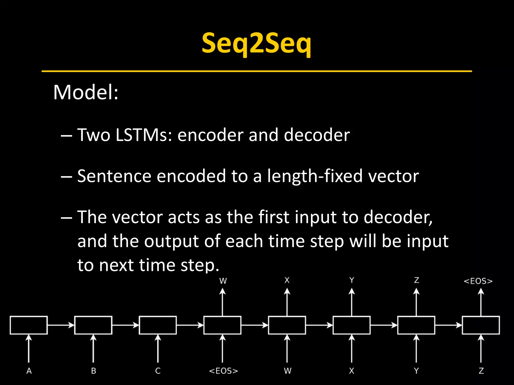
 Model:
– Two LSTMs: encoder and decoder
– Sentence encoded to a length-fixed vector
– The vector acts as the first input to decoder,
and the output of each time step will be input
to next time step.
Seq2Seq
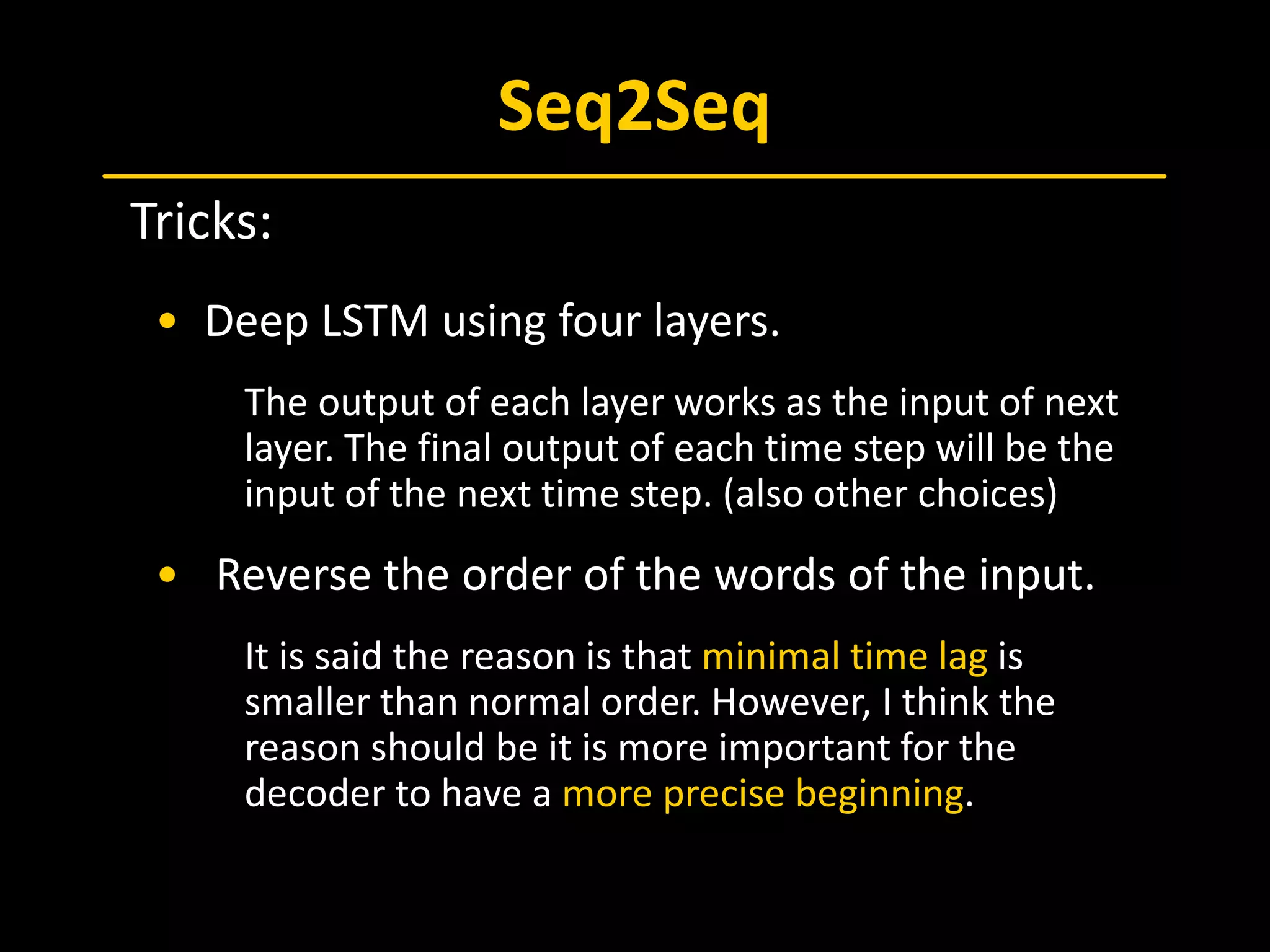
 Tricks:
• Deep LSTM using four layers.
The output of each layer works as the input of next
layer. The final output of each time step will be the
input of the next time step. (also other choices)
• Reverse the order of the words of the input.
It is said the reason is that minimal time lag is
smaller than normal order. However, I think the
reason should be it is more important for the
decoder to have a more precise beginning.
Attention
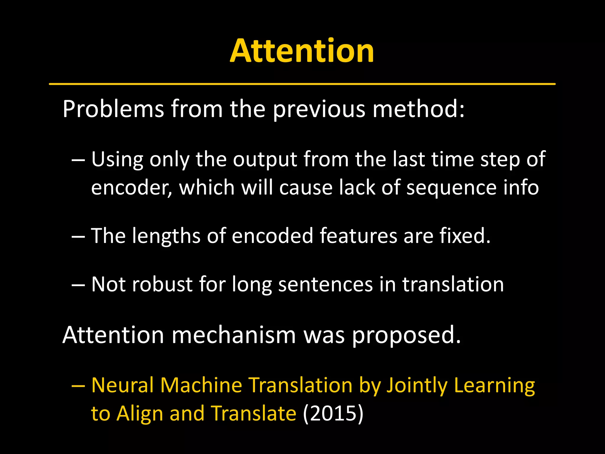
 Problems from the previous method:
– Using only the output from the last time step of
encoder, which will cause lack of sequence info
– The lengths of encoded features are fixed.
– Not robust for long sentences in translation
 Attention mechanism was proposed.
– Neural Machine Translation by Jointly Learning
to Align and Translate (2015)
Attention
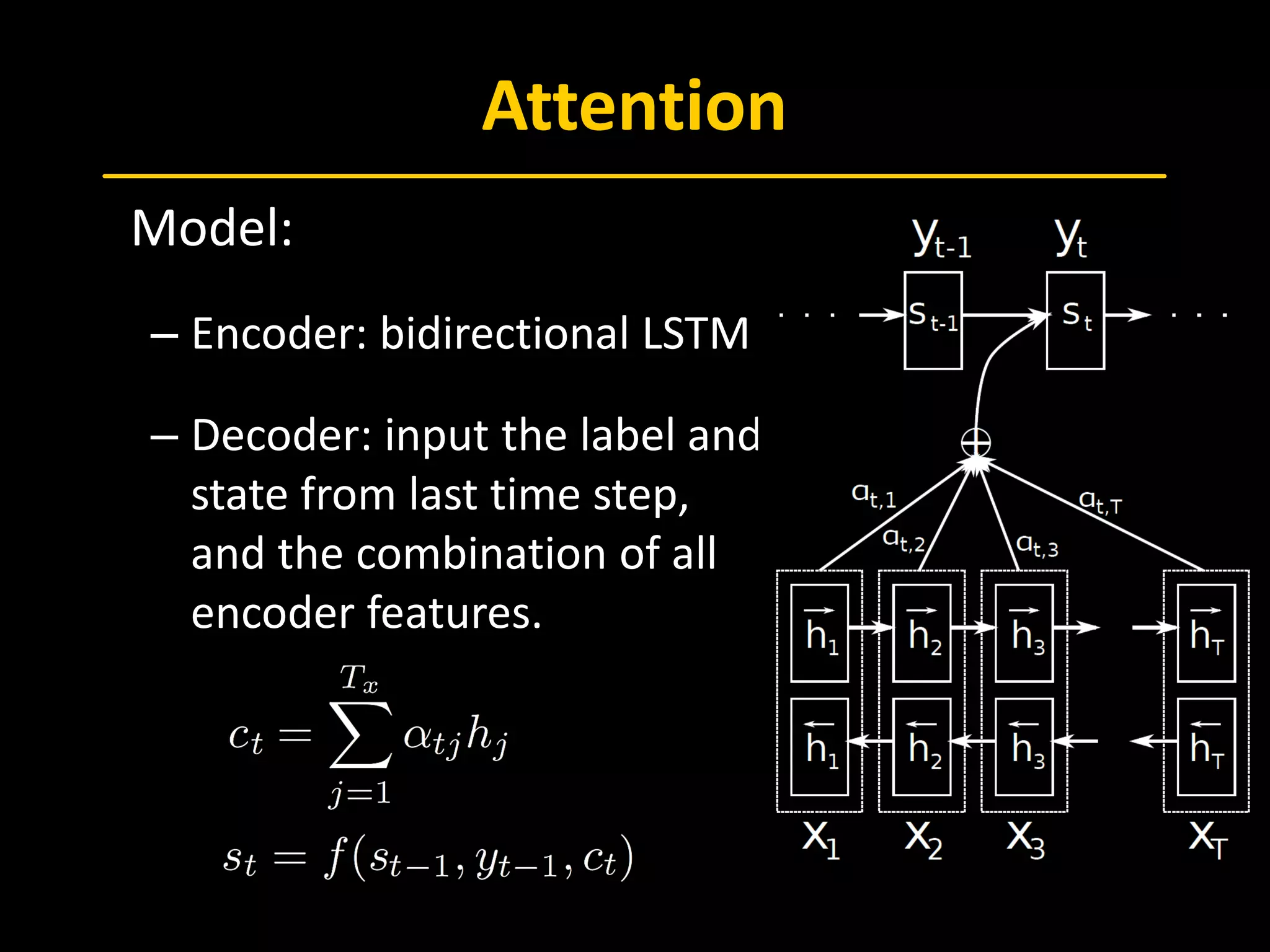
 Model:
– Encoder: bidirectional LSTM
– Decoder: input the label and
state from last time step,
and the combination of all
encoder features.
Attention
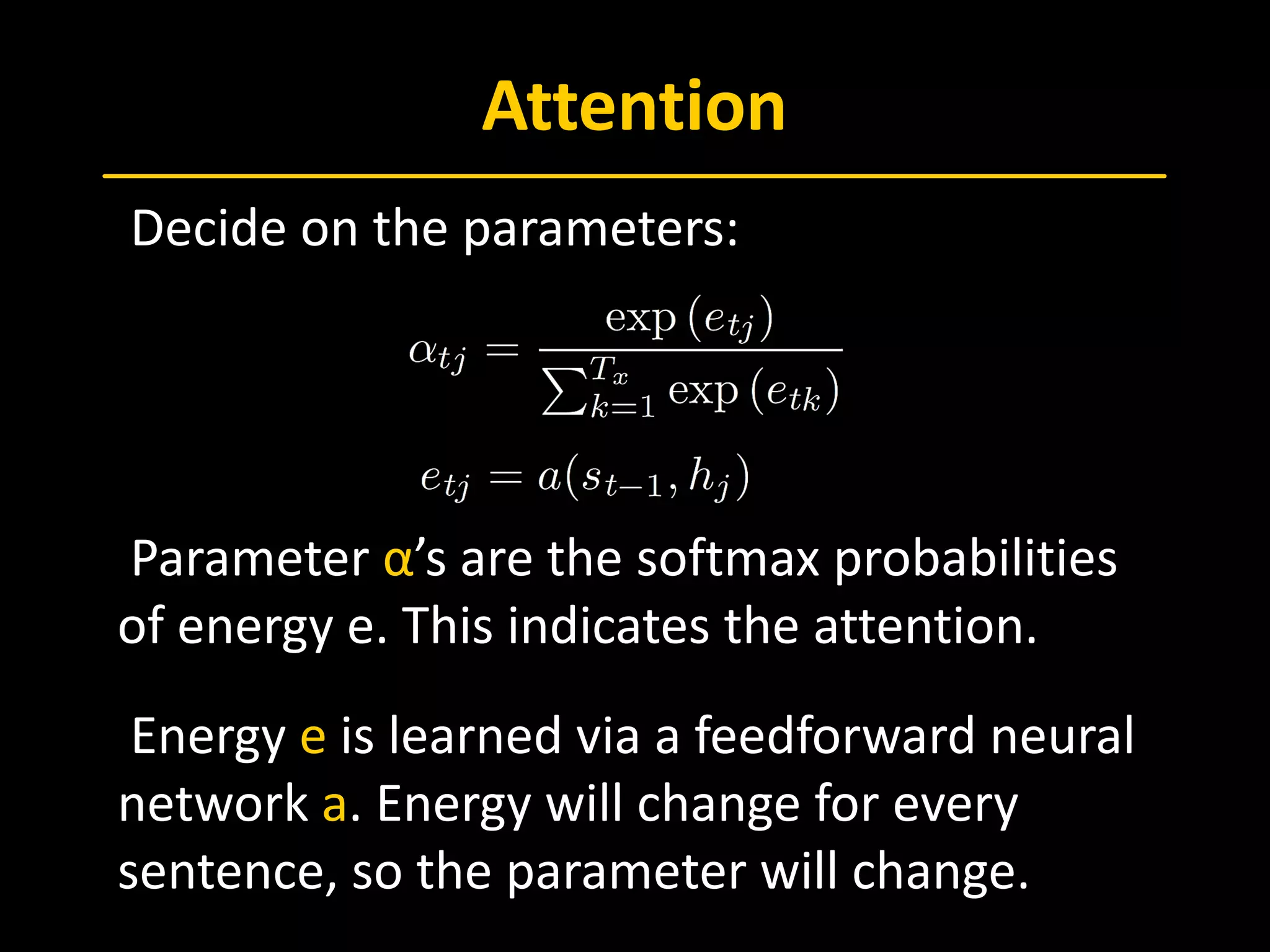
 Decide on the parameters:
 Parameter α’s are the softmax probabilities
of energy e. This indicates the attention.
 Energy e is learned via a feedforward neural
network a. Energy will change for every
sentence, so the parameter will change.
Image Captioning
 If we exchange the encoder to CNN to deal
with images, the structure will transfer
information from image to language, which is
the idea of image captioning.
– Show, Attend and Tell Neural Image Caption
Generation with Visual Attention (2015)
– Boosting Image Captioning with Attributes (2017)
– Describing Videos by Exploiting Temporal
Structure (2015)
Image Captioning
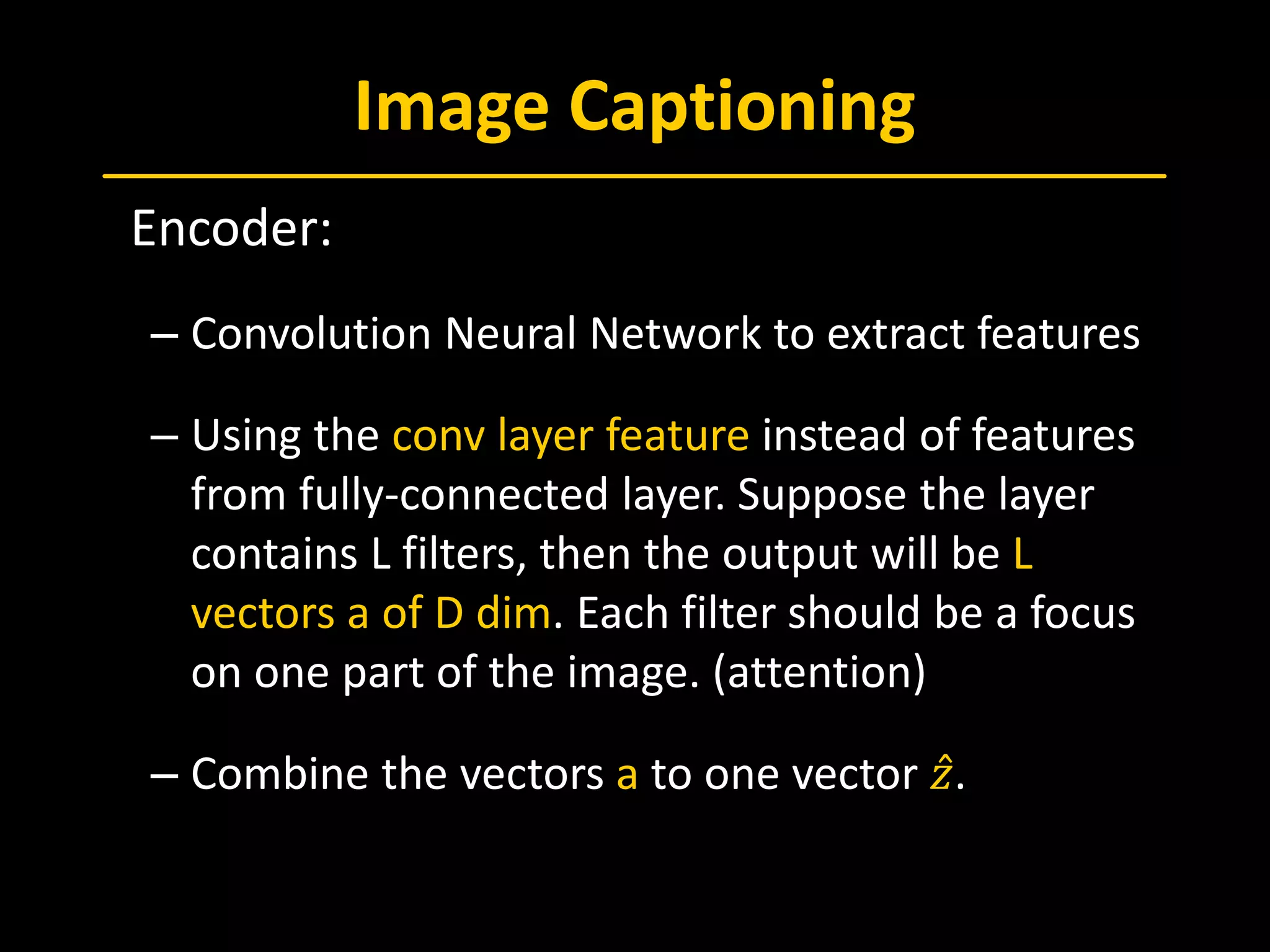
 Encoder:
– Convolution Neural Network to extract features
– Using the conv layer feature instead of features
from fully-connected layer. Suppose the layer
contains L filters, then the output will be L
vectors a of D dim. Each filter should be a focus
on one part of the image. (attention)
– Combine the vectors a to one vector 𝑧𝑧̂.
Image Captioning
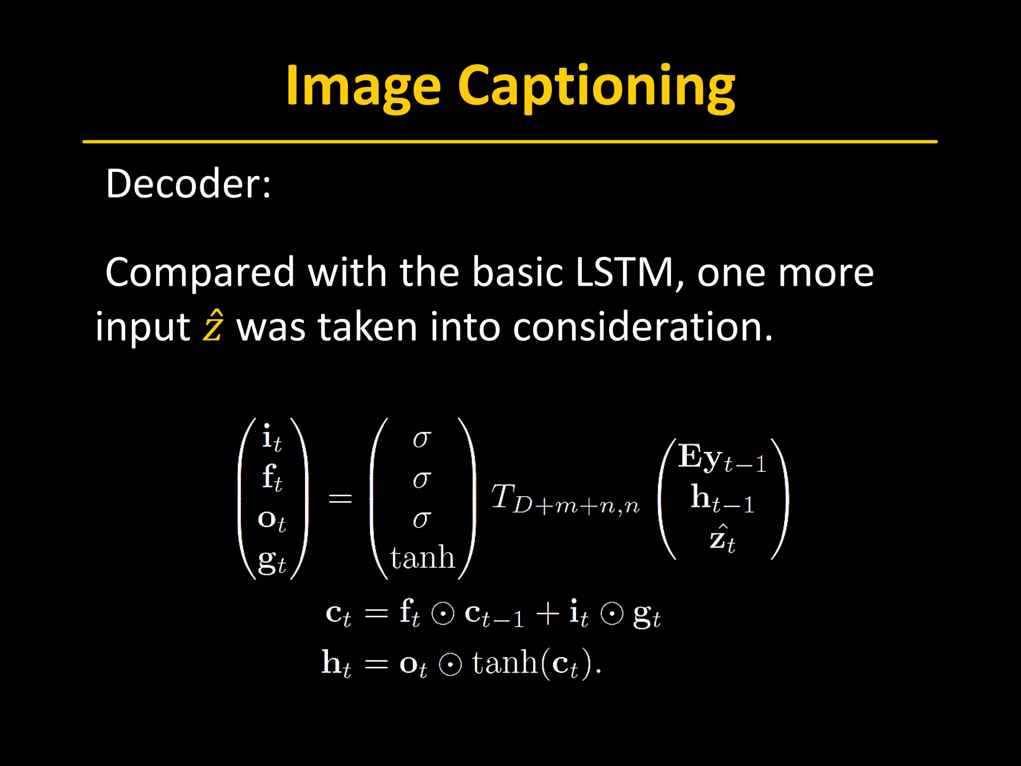
 Decoder:
 Compared with the basic LSTM, one more
input 𝑧𝑧̂ was taken into consideration.
Image Captioning
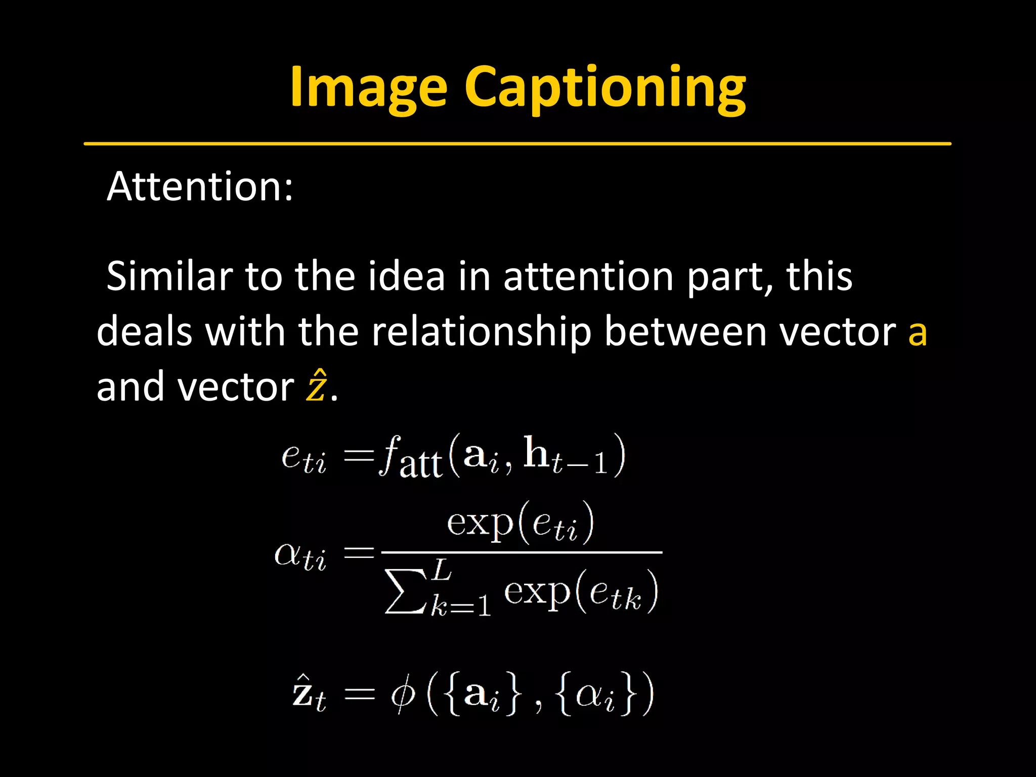
 Attention:
 Similar to the idea in attention part, this
deals with the relationship between vector a
and vector 𝑧𝑧̂.
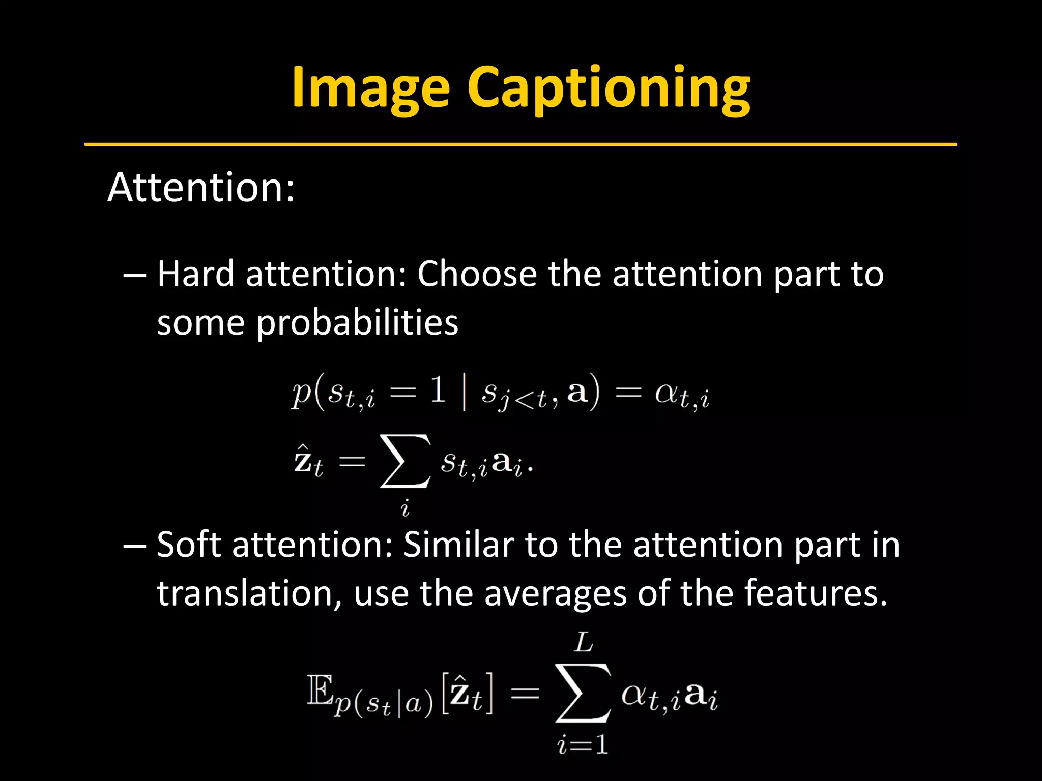
Image Captioning
 Attention:
– Hard attention: Choose the attention part to
some probabilities
– Soft attention: Similar to the attention part in
translation, use the averages of the features.
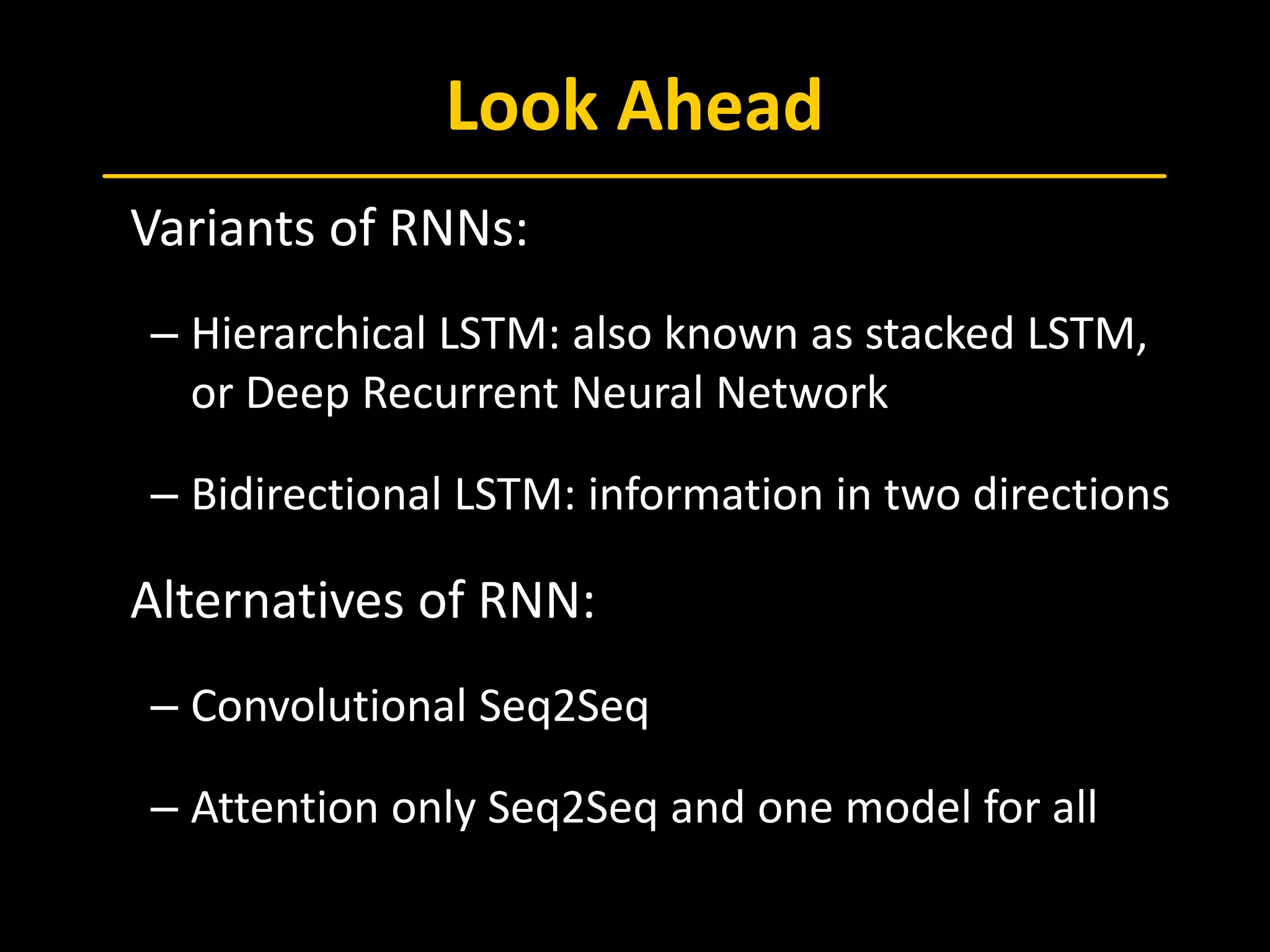
Look Ahead
 Variants of RNNs:
– Hierarchical LSTM: also known as stacked LSTM,
or Deep Recurrent Neural Network
– Bidirectional LSTM: information in two directions
 Alternatives of RNN:
– Convolutional Seq2Seq
– Attention only Seq2Seq and one model for all
References
[Goodfellow, 2016] Goodfellow, I., Bengio, Y., & Courville, A. (2016). Deep le
arning. MIT press.
[Sutskever, 2014] Sutskever, I., Vinyals, O., & Le, Q. V. (2014). Sequence to se
quence learning with neural networks. In Advances in neural information pr
ocessing systems (pp. 3104-3112).
[Bahdanau, 2014] Bahdanau, D., Cho, K., & Bengio, Y. (2014). Neural machin
e translation by jointly learning to align and translate. arXiv preprint arXiv:1
409.0473. ICLR 2015
[Yao, 2016] Yao, Ting, Pan, Yingwei, Li, Yehao, Qiu, Zhaofan, & Mei, Tao. (201
6). Boosting image captioning with attributes. ICLR 2017
[Xu, 2015] Xu, K., Ba, J., Kiros, R., Cho, K., Courville, A., & Salakhutdinov, R., e
t al. (2015). Show, attend and tell: neural image caption generation with vis
ual attention. Computer Science, 2048-2057.
[Yao, 2015] Yao L, Torabi A, Cho K, et al. Describing Videos by Exploiting Tem
poral Structure[J]. Eprint Arxiv, 2015, 53:199-211.
References
[Chollet, 2016] Chollet, F. (2016). Xception: Deep Learning with Depthwise S
eparable Convolutions. arXiv preprint arXiv:1610.02357.
[Gehring, 2017] Gehring, J., Auli, M., Grangier, D., Yarats, D., & Dauphin, Y. N.
(2017). Convolutional Sequence to Sequence Learning. arXiv preprint arXiv:
1705.03122.
[Vaswani, 2017] Vaswani, A., Shazeer, N., Parmar, N., Uszkoreit, J., Jones, L.,
Gomez, A. N., ... & Polosukhin, I. (2017). Attention Is All You Need. arXiv pre
print arXiv:1706.03762.
[Kaiser, 2017] Kaiser, L., Gomez, A. N., Shazeer, N., Vaswani, A., Parmar, N., J
ones, L., & Uszkoreit, J. (2017). One Model To Learn Them All. arXiv preprint
arXiv:1706.05137.

RNN and sequence-to-sequence processing

  • 1.
    RNN, Seq2Seq Learning andImage Captioning Dongang Wang 07 July 2017
  • 2.
    Contents • From RNNto LSTM • Backpropagation through time (BPTT) • Usage of LSTM • Seq2Seq Learning • Attention Mechanism • Image Captioning
  • 3.
  • 4.
    Recurrent Neural Network  Thefollowing update equations:  with the cross entropy loss:
  • 5.
    Backpropagation Through Time  Usingthe previous equations, we could find the derivatives of loss over the parameters:  The s stands for the sizes of each part. Specially, , which means the function  does not change the dimensions. 1 1 , , , a x o h a h a o s s s s s s s s U V W b c × × × × × ∈ ∈ ∈ ∈ ∈      2 2 1 tanh( ) 1 x x x x x x e e e x e e e − − − − = = + + a hs s=
  • 6.
    Backpropagation Through Time  Step1: understand loss  we have  which means for any parameter M:  In that case, we could only deal with one time step. , ,a x a x a xs s s s s s U U U× × × ∈ ∈ ∈   ( ) 1t L L ∂ = ∂ ( ) ( ) t t t L L L M L M ∂ ∂ ∂ = ∂ ∂ ∂ ∑
  • 7.
    Backpropagation Through Time  Step1: understand loss  We assume that the labels are one-hot, so the loss for each time step should be  Only m-th element left. And we will have T( ) ( )( ) ( ) ( ) T ( ) ( ) ( ) ˆlog 0,0,... ,...,0,0 ˆ ˆ 1 0,0,... ,...,0,0 ˆ ˆ t tt m m t t m t t t m y yL y y y y y  −∂∂ =   ∂ ∂   − = = −   
  • 8.
    Backpropagation Through Time  Step2: derivatives of V and c  Straightforward: ( ) ( ) ( ) ( ) ( ) ( ) ( ) ( ) ( ) ( ) ( ) ( ) ˆ ˆ ˆ ˆ t t t t t t t t t t t t L L y o V y o V L L y o c y o c ∂ ∂ ∂ ∂ = ⋅ ⋅ ∂ ∂ ∂ ∂ ∂ ∂ ∂ ∂ = ⋅ ⋅ ∂ ∂ ∂ ∂ ( ) ( ) ( ) , and 1 T t t to o h V c ∂ ∂ = = ∂ ∂
  • 9.
    Backpropagation Through Time  Step2: derivatives of V and c  The derivative of softmax:  and i j x x e y e = ∑( )( ) 1 ( ) ( ) 1 1( ) ( ) ( )( ) 1 ( ) ( ) ˆˆ ˆ = ˆˆ tt d t t t t tt d t t d d yy o o y o yy o o  ∂∂   ∂ ∂  ∂    ∂ ∂∂   ∂ ∂       ( ) ( ) ( )( ) ( ) ( ) ( ) ˆ ˆ ˆ , ifˆ = ˆ ˆ , if t t tt i i ii t t t j i j y y y i jy o y y i j  − =∂   ∂ ≠
  • 10.
    Backpropagation Through Time  Step2: derivatives of V and c  Since we have , which will pick up one column from the above matrix, the result will be: T ( ) ( ) ( ) 1 0,0,... ,...,0,0 ˆ ˆ t t t m L y y  ∂ − =   ∂   ( )( ) 1 ( ) ( ) T 1 1( ) ( ) ( ) ( ) ( ) ( ) ( ) ( )( ) 1 ( ) ( ) T( ) ( ) ( ) ( ) ( ) ( ) 1 2 ˆˆ ˆ 1 = 0,0,... ,...,0,0 ˆ ˆ ˆˆ ˆ ˆ ˆ ˆ ˆ, ,..., 1,..., tt d t t t t t t t t t m tt d t t d d t t t t t t m d yy o o L L y o y o y yy o o y y y y y y  ∂∂   ∂ ∂  ∂ ∂ ∂ −  =    ∂ ∂ ∂   ∂∂   ∂ ∂   = − =−      
  • 11.
    Backpropagation Through Time  Step2: derivatives of V and c  We have already got    so: ( ) ( ) ( ) ( ) ( ) ( ) ( ) ( ) ( ) ( ) ( ) ( ) ( ) ( ) ( ) ˆ ˆ( ) ˆ ˆ ˆ( ) ˆ T t t t t t t t t t t t t t t t t t t t L L y o y y h V y o V L L y o y y c y o c ∂ ∂ ∂ ∂ = ⋅ ⋅ = − ⋅ ∂ ∂ ∂ ∂ ∂ ∂ ∂ ∂ = ⋅ ⋅ = − ∂ ∂ ∂ ∂ ∑ ∑ ∑ ∑ ( ) ( ) ( ) , and 1 T t t to o h V c ∂ ∂ = ∂ ∂ ( ) ( ) ( ) ( ) ( ) ( ) ( ) ( ) ˆ ˆ ˆ t t t t t t t t L L y y y o y o ∂ ∂ ∂ = = − ∂ ∂ ∂
  • 12.
    Backpropagation Through Time  Step3: derivatives of h  We already have  and ( ) ( ) ( ) ( ) ( 1) ( 1) ( ) ( ) ( ) ( 1) ( 1) ( ) t t t t t t t t t t t t L L o L h a h o h h a h + + + + ∂ ∂ ∂ ∂ ∂ ∂ = ⋅ + ⋅ ⋅ ∂ ∂ ∂ ∂ ∂ ∂ ( ) ( ) ( ) ( ) ( ) ( ) ( ) ( ) ˆ ˆ ˆ t t t t t t t t L L y y y o y o ∂ ∂ ∂ = = − ∂ ∂ ∂ ( ) ( 1) ( ) ( ) , and T T t t t t o a V W h h + ∂ ∂ = = ∂ ∂
  • 13.
    Backpropagation Through Time  Step3: derivatives of h  The derivative of tanh:  we have observed that  so 2 2 tanh( ) 4 2x x d x dx e e− = + + 2 2 2 2 2 2 2 2 4 tanh ( ) 1 2 2 x x x x x x e e x e e e e − − − + − = = − + + + + 2tanh( ) 1 tanh ( ) d x x dx = −
  • 14.
    Backpropagation Through Time  Step3: derivatives of h  Combine all the above together:  Until the last time step
  • 15.
    Backpropagation Through Time  Step4: derivatives of U, W and b  We can write:  and we have ( ) ( ) ( ) ( ) ( ) ( ) ( ) ( ) ( ) ( ) ( ) ( ) ( ) ( ) ( ) ( ) ( ) ( ) t t t t t t t t t t t t t t t t t t L L h a b h a b L L h a U h a U L L h a W h a W ∂ ∂ ∂ ∂ = ⋅ ⋅ ∂ ∂ ∂ ∂ ∂ ∂ ∂ ∂ = ⋅ ⋅ ∂ ∂ ∂ ∂ ∂ ∂ ∂ ∂ = ⋅ ⋅ ∂ ∂ ∂ ∂ ( ) ( ) ( ) ( 1) ( ) 1, , and T T t t t t ta a a h x b W U −∂ ∂ ∂ = = = ∂ ∂ ∂
  • 16.
  • 17.
  • 18.
    Long-term Dependency  This isan inherent problem, like Gradient Vanishing Problem in CNN.  Let’s focus on the hidden state. Somehow it just works as matrix multiplication:  The state of last step according to the first:
  • 19.
    Long-term Dependency  If wetake the eigendecomposition of the above equation:  This means the eigenvalues should not be too large or too small, or the hidden states after several steps will be vanished or exaggerated. The ideal choice should be ≈1.
  • 20.
    Long Short TermMemory  LSTM was proposed in 1997, which is designed to add some variances to the net.   sigmoid   tanh
  • 21.
    Long Short TermMemory  i  input gate, f  forget gate,  o  output gate, g  input modulation,  z  output, h  state, c  memory cell
  • 22.
    Usage of RNN(LSTM)  Oneinput, Many output • Image Captioning • Language Translation  Many input, One output • Video Classification • Language Classification  Many input, Many output • Language Translation • Video Captioning
  • 23.
    Seq2Seq  One successful implementationof LSTM is Sequence-to-Sequence learning. This is first introduced to solve machine translation problems (kind of transfer learning). – Sequence to sequence learning with neural networks (2014) – Learning Phrase Representation using RNN Encoder-Decoder for Statistical Machine Translation (2014)
  • 24.
    Seq2Seq  NLP fundations: • wordembedding There are two ways to represent word. One is using dictionary, and each word will be a one-hot vector. The other way is using word embedding tools like word2vec. • beam searching For output, each time there will be an output of softmax probabilities. It is not fair to choose the word with largest prob as the prediction. Instead, we choose k largest each time, where k is the beam size.
  • 25.
    Seq2Seq  Model: – Two LSTMs:encoder and decoder – Sentence encoded to a length-fixed vector – The vector acts as the first input to decoder, and the output of each time step will be input to next time step.
  • 26.
    Seq2Seq  Tricks: • Deep LSTMusing four layers. The output of each layer works as the input of next layer. The final output of each time step will be the input of the next time step. (also other choices) • Reverse the order of the words of the input. It is said the reason is that minimal time lag is smaller than normal order. However, I think the reason should be it is more important for the decoder to have a more precise beginning.
  • 27.
    Attention  Problems from theprevious method: – Using only the output from the last time step of encoder, which will cause lack of sequence info – The lengths of encoded features are fixed. – Not robust for long sentences in translation  Attention mechanism was proposed. – Neural Machine Translation by Jointly Learning to Align and Translate (2015)
  • 28.
    Attention  Model: – Encoder: bidirectionalLSTM – Decoder: input the label and state from last time step, and the combination of all encoder features.
  • 29.
    Attention  Decide on theparameters:  Parameter α’s are the softmax probabilities of energy e. This indicates the attention.  Energy e is learned via a feedforward neural network a. Energy will change for every sentence, so the parameter will change.
  • 30.
    Image Captioning  If weexchange the encoder to CNN to deal with images, the structure will transfer information from image to language, which is the idea of image captioning. – Show, Attend and Tell Neural Image Caption Generation with Visual Attention (2015) – Boosting Image Captioning with Attributes (2017) – Describing Videos by Exploiting Temporal Structure (2015)
  • 31.
    Image Captioning  Encoder: – ConvolutionNeural Network to extract features – Using the conv layer feature instead of features from fully-connected layer. Suppose the layer contains L filters, then the output will be L vectors a of D dim. Each filter should be a focus on one part of the image. (attention) – Combine the vectors a to one vector 𝑧𝑧̂.
  • 32.
    Image Captioning  Decoder:  Compared withthe basic LSTM, one more input 𝑧𝑧̂ was taken into consideration.
  • 33.
    Image Captioning  Attention:  Similar tothe idea in attention part, this deals with the relationship between vector a and vector 𝑧𝑧̂.
  • 34.
    Image Captioning  Attention: – Hardattention: Choose the attention part to some probabilities – Soft attention: Similar to the attention part in translation, use the averages of the features.
  • 35.
    Look Ahead  Variants ofRNNs: – Hierarchical LSTM: also known as stacked LSTM, or Deep Recurrent Neural Network – Bidirectional LSTM: information in two directions  Alternatives of RNN: – Convolutional Seq2Seq – Attention only Seq2Seq and one model for all
  • 36.
    References [Goodfellow, 2016] Goodfellow,I., Bengio, Y., & Courville, A. (2016). Deep le arning. MIT press. [Sutskever, 2014] Sutskever, I., Vinyals, O., & Le, Q. V. (2014). Sequence to se quence learning with neural networks. In Advances in neural information pr ocessing systems (pp. 3104-3112). [Bahdanau, 2014] Bahdanau, D., Cho, K., & Bengio, Y. (2014). Neural machin e translation by jointly learning to align and translate. arXiv preprint arXiv:1 409.0473. ICLR 2015 [Yao, 2016] Yao, Ting, Pan, Yingwei, Li, Yehao, Qiu, Zhaofan, & Mei, Tao. (201 6). Boosting image captioning with attributes. ICLR 2017 [Xu, 2015] Xu, K., Ba, J., Kiros, R., Cho, K., Courville, A., & Salakhutdinov, R., e t al. (2015). Show, attend and tell: neural image caption generation with vis ual attention. Computer Science, 2048-2057. [Yao, 2015] Yao L, Torabi A, Cho K, et al. Describing Videos by Exploiting Tem poral Structure[J]. Eprint Arxiv, 2015, 53:199-211.
  • 37.
    References [Chollet, 2016] Chollet,F. (2016). Xception: Deep Learning with Depthwise S eparable Convolutions. arXiv preprint arXiv:1610.02357. [Gehring, 2017] Gehring, J., Auli, M., Grangier, D., Yarats, D., & Dauphin, Y. N. (2017). Convolutional Sequence to Sequence Learning. arXiv preprint arXiv: 1705.03122. [Vaswani, 2017] Vaswani, A., Shazeer, N., Parmar, N., Uszkoreit, J., Jones, L., Gomez, A. N., ... & Polosukhin, I. (2017). Attention Is All You Need. arXiv pre print arXiv:1706.03762. [Kaiser, 2017] Kaiser, L., Gomez, A. N., Shazeer, N., Vaswani, A., Parmar, N., J ones, L., & Uszkoreit, J. (2017). One Model To Learn Them All. arXiv preprint arXiv:1706.05137.