UNIVERSITY OF MEDICAL SCIENCE AND TECHNOLOGY
FACULTY OF PHARMACY
DEPARTMENT OF PHARMACEUTICAL CHEMISTRY
M.Sc. Pharmaceutical Analysis and Quality Control
Semester 2
Subject: Total Quality Management
Topic: Different types of Histogram
By: Supervisor
Mohamed Hersi Farah Dr. Sophia Sahal Elmardi
Khartoum-Sudan
08-april-2019
Introduction:
A histogram is used to summarize discrete or continuous data. In other words, it
provides a visual interpretation of numerical data by showing the number of data
points that fall within a specified range of values (called “bins”). It is similar to a
vertical bar graph. However, a histogram, unlike a vertical bar graph, shows no
gaps between the bars.
Figure 1: Histogram
Parts of a Histogram
1. The title: The title describes the information included in the histogram.
2. X-axis: The X-axis are intervals that show the scale of values in which the
measurements fall under.
3. Y-axis: The Y-axis shows the number of times that the values occurred
within the intervals set by the X-axis.
4. The bars: The height of the bar shows the number of times that the values
occurred within the interval while the width of the bar shows the interval
that is covered. For a histogram with equal bins, the width should be the
same across all bars.
Importance of a Histogram
Creating a histogram provides a visual representation of data distribution.
Histograms display a large amount of data and the frequency of the data values.
The median and distribution of the data can be determined by a histogram. In
addition, it can show any outliers or gaps in the data.
Distributions of a Histogram:
A normal distribution: In a normal distribution, points on one side of the average
are as likely to occur as on the other side of the average.
Figure 2: Normal Distribution
A bimodal distribution: In a bimodal distribution, there are two peaks. In a
bimodal distribution, the data should be separated and analyzed as separate normal
distributions.
Figure 3: bimodal distribution
A right-skewed distribution: A right-skewed distribution is also called a
positively skewed distribution. In a right-skewed distribution, a large number of
the data values occur on the left side with a fewer number of data values on the
right side. A right-skewed distribution usually occurs when the data has a range
boundary on the left-hand side of the histogram. For example, a boundary of 0.
Figure 4: right-skewed distribution
A left-skewed distribution: A left-skewed distribution is also called a negatively
skewed distribution. In a left-skewed distribution, a large number of the data
values occur on the right side with a fewer number of data values on the left side.
A right-skewed distribution usually occurs when the data has a range boundary on
the right-hand side of the histogram. For example, a boundary such as 100.
Figure 5: left-skewed distribution
A random distribution: A random distribution lacks an apparent pattern and has
several peaks. In a random-distribution histogram, it can be the case that different
data properties were combined. Therefore, the data should be separated and
analyzed separately.
Figure 6: Random Distribution
Standard types of histograms:
In many cases, the histogram is skewed to one side or may have more than one
peak (e.g., exam grades often produce a strange-looking histogram).
There are five standard histogram shapes that have been given standardized
names:
 Symmetric: Nearly symmetric left to right, with a peak very close to the middle.
Figure 7a: (Symmetric) Figure 7b: (Symmetric, unimodal)
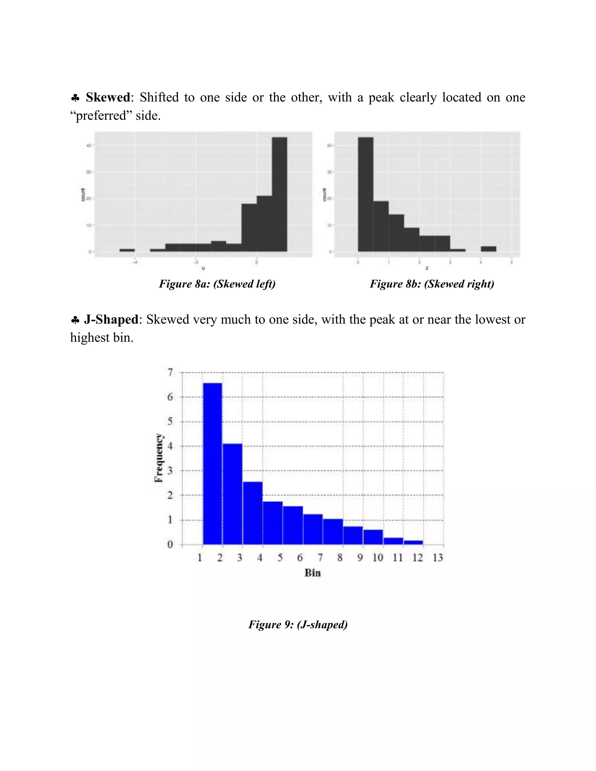
 Skewed: Shifted to one side or the other, with a peak clearly located on one
“preferred” side.
Figure 8a: (Skewed left) Figure 8b: (Skewed right)
 J-Shaped: Skewed very much to one side, with the peak at or near the lowest or
highest bin.
Figure 9: (J-shaped)
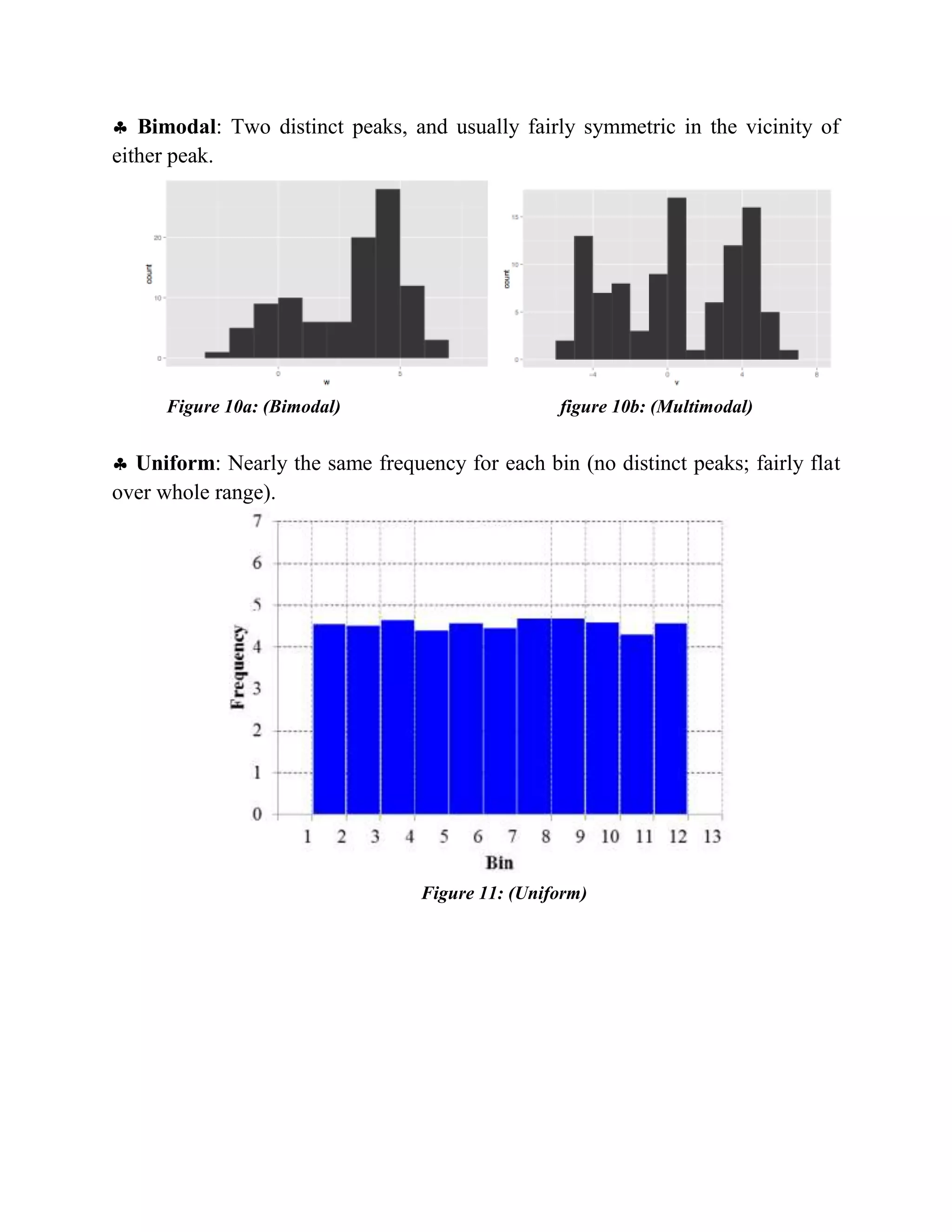
 Bimodal: Two distinct peaks, and usually fairly symmetric in the vicinity of
either peak.
Figure 10a: (Bimodal) figure 10b: (Multimodal)
 Uniform: Nearly the same frequency for each bin (no distinct peaks; fairly flat
over whole range).
Figure 11: (Uniform)

Research differen tyes of histogram

  • 1.
    UNIVERSITY OF MEDICALSCIENCE AND TECHNOLOGY FACULTY OF PHARMACY DEPARTMENT OF PHARMACEUTICAL CHEMISTRY M.Sc. Pharmaceutical Analysis and Quality Control Semester 2 Subject: Total Quality Management Topic: Different types of Histogram By: Supervisor Mohamed Hersi Farah Dr. Sophia Sahal Elmardi Khartoum-Sudan 08-april-2019
  • 2.
    Introduction: A histogram isused to summarize discrete or continuous data. In other words, it provides a visual interpretation of numerical data by showing the number of data points that fall within a specified range of values (called “bins”). It is similar to a vertical bar graph. However, a histogram, unlike a vertical bar graph, shows no gaps between the bars. Figure 1: Histogram Parts of a Histogram 1. The title: The title describes the information included in the histogram. 2. X-axis: The X-axis are intervals that show the scale of values in which the measurements fall under. 3. Y-axis: The Y-axis shows the number of times that the values occurred within the intervals set by the X-axis. 4. The bars: The height of the bar shows the number of times that the values occurred within the interval while the width of the bar shows the interval that is covered. For a histogram with equal bins, the width should be the same across all bars. Importance of a Histogram Creating a histogram provides a visual representation of data distribution. Histograms display a large amount of data and the frequency of the data values. The median and distribution of the data can be determined by a histogram. In addition, it can show any outliers or gaps in the data. Distributions of a Histogram: A normal distribution: In a normal distribution, points on one side of the average are as likely to occur as on the other side of the average. Figure 2: Normal Distribution
  • 3.
    A bimodal distribution:In a bimodal distribution, there are two peaks. In a bimodal distribution, the data should be separated and analyzed as separate normal distributions. Figure 3: bimodal distribution A right-skewed distribution: A right-skewed distribution is also called a positively skewed distribution. In a right-skewed distribution, a large number of the data values occur on the left side with a fewer number of data values on the right side. A right-skewed distribution usually occurs when the data has a range boundary on the left-hand side of the histogram. For example, a boundary of 0. Figure 4: right-skewed distribution A left-skewed distribution: A left-skewed distribution is also called a negatively skewed distribution. In a left-skewed distribution, a large number of the data values occur on the right side with a fewer number of data values on the left side. A right-skewed distribution usually occurs when the data has a range boundary on the right-hand side of the histogram. For example, a boundary such as 100. Figure 5: left-skewed distribution
  • 4.
    A random distribution:A random distribution lacks an apparent pattern and has several peaks. In a random-distribution histogram, it can be the case that different data properties were combined. Therefore, the data should be separated and analyzed separately. Figure 6: Random Distribution Standard types of histograms: In many cases, the histogram is skewed to one side or may have more than one peak (e.g., exam grades often produce a strange-looking histogram). There are five standard histogram shapes that have been given standardized names:  Symmetric: Nearly symmetric left to right, with a peak very close to the middle. Figure 7a: (Symmetric) Figure 7b: (Symmetric, unimodal)
  • 5.
     Skewed: Shiftedto one side or the other, with a peak clearly located on one “preferred” side. Figure 8a: (Skewed left) Figure 8b: (Skewed right)  J-Shaped: Skewed very much to one side, with the peak at or near the lowest or highest bin. Figure 9: (J-shaped)
  • 6.
     Bimodal: Twodistinct peaks, and usually fairly symmetric in the vicinity of either peak. Figure 10a: (Bimodal) figure 10b: (Multimodal)  Uniform: Nearly the same frequency for each bin (no distinct peaks; fairly flat over whole range). Figure 11: (Uniform)