Probability
Probability is the chance of an outcome in an experiment (also called event).
Event: Tossing a fair coin
Outcome: Head, Tail
Probability deals with predicting the likelihood of future events.
Probability Distribution: It is a listing of the probabilities of all the possible
outcomes that could occur if the experiment was done.
OR
A probability distribution is a definition of probabilities of the values of random
variable.
OR
The relationship between the values of a random variable and the probability of
their occurrence summarized by means of a device called a probability distribution.
It may be expressed in the form of a table, a graph or a formula.
Knowledge of probability distribution of a random variable provides the
researchers with a powerful tool for summarizing and describing a set of data and
for reaching conclusion about a population on the basis of sample.
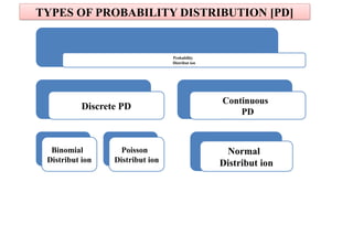
TYPES OF PROBABILITY DISTRIBUTION [PD]
Probability
Distribut ion
Discrete PD
Binomial
Distribut ion
Poisson
Distribut ion
Continuous
PD
Normal
Distribut ion
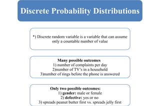
Discrete Probability Distributions
*) Discrete random variable is a variable that can assume
only a countable number of value
Many possible outcomes
1) number of complaints per day
2)number of TV’s in a household
3)number of rings before the phone is answered
Only two possible outcomes:
1) gender: male or female
2) defective: yes or no
3) spreads peanut butter first vs. spreads jelly first
Binomial distribution was discovered by James Bernoulli (1654-1705).
There are certain phenomena in nature which can be identified as
Bernoulli’s processes, in which:
There is a fixed number of n trials carried out
Each trial has only two possible outcomes say success or failure,
true or false etc.
Probability of occurrence of any outcome remains same over
successive trials
Trials are statistically independent
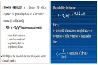
 A random experiment be performed repeatedly and the occurrence of
an event in a trial be called as success and its non-occurrence is failure.
Consider a set of n independent trails (n being finite), in which the
probability p of success in any trail is constant for each trial.
Then q=1-p is the probability of failure in any trail.
BINOMIAL DISTRIBUTION
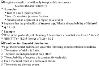
Imagine a simple trial with only two possible outcomes:-
Success (S) and Failure (F)
 Examples
Toss of a coin (heads or tails)
Sex of a newborn (male or female)
Survival of an organism in a region (live or die)
Suppose that the probability of success is p, What is the probability of failure?
 q = 1 – p
Example
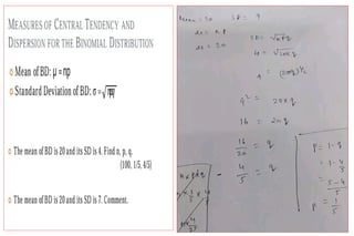
What is the probability of obtaining 2 heads from a coin that was tossed 5 times?
P(HHTTT) = (1/2)5 (power of 1/2) = 1/32
Condition for Binomial distribution
We get the binomial distribution under the following experimentation conditions
1. The number of trial n is finite
2. The trials are independent of each other.
3. The probability of success p is constant for each trial.
4. Each trial must result in a success or failure.
5. The events are discrete events.
Ashish
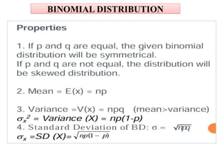
BINOMIAL DISTRIBUTION
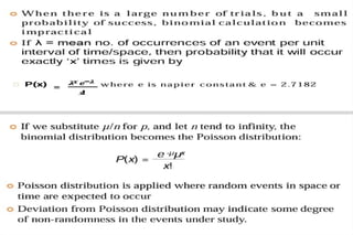
When there is a large number of trials, but a small probability of success,
binomial calculation becomes impractical.
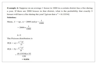
Example: Number of deaths from horse kicks in the Army in different
years
Example: 64 deaths in 20 years from thousands of soldiers
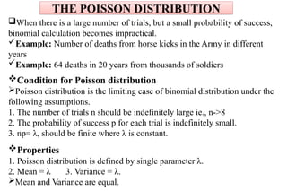
Condition for Poisson distribution
Poisson distribution is the limiting case of binomial distribution under the
following assumptions.
1. The number of trials n should be indefinitely large ie., n->8
2. The probability of success p for each trial is indefinitely small.
3. np= λ, should be finite where λ is constant.
Properties
1. Poisson distribution is defined by single parameter λ.
2. Mean = λ 3. Variance = λ.
Mean and Variance are equal.
THE POISSON DISTRIBUTION
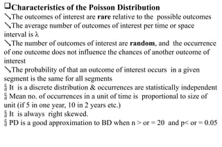
Characteristics of the Poisson Distribution
The outcomes of interest are rare relative to the possible outcomes
The average number of outcomes of interest per time or space
interval is λ
The number of outcomes of interest are random, and the occurrence
of one outcome does not influence the chances of another outcome of
interest
The probability of that an outcome of interest occurs in a given
segment is the same for all segments
 It is a discrete distribution & occurrences are statistically independent
 Mean no. of occurrences in a unit of time is proportional to size of
unit (if 5 in one year, 10 in 2 years etc.)
 It is always right skewed.
 PD is a good approximation to BD when n > or = 20 and p< or = 0.05
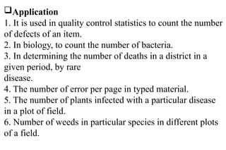
Application
1. It is used in quality control statistics to count the number
of defects of an item.
2. In biology, to count the number of bacteria.
3. In determining the number of deaths in a district in a
given period, by rare
disease.
4. The number of error per page in typed material.
5. The number of plants infected with a particular disease
in a plot of field.
6. Number of weeds in particular species in different plots
of a field.
NORMAL DISTRIBUTION
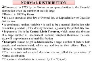
Discovered in 1733 by de Moivre as an approximation to the binomial
distribution when the number of trails is large
Derived in 1809 by Gauss
It is also known as error law or Normal law or Laplacian law or Gaussian
distribution.
A continuous random variable x is said to be a normal distribution with
parameters µ and σ2 , if the density function is given by the probability law.
Importance lies in the Central Limit Theorem, which states that the sum
of a large number of independent random variables (binomial, Poisson,
etc.) will approximate a normal distribution
Example: Human height is determined by a large number of factors, both
genetic and environmental, which are additive in their effects. Thus, it
follows a normal distribution.
The mean (m) and standard deviation (s) are called the parameters of
Normal distribution.
The normal distribution is expressed by X ~ N(m, σ2)
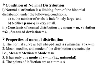
Condition of Normal Distribution
i) Normal distribution is a limiting form of the binomial
distribution under the following conditions.
a) n, the number of trials is indefinitely large and
b) Neither p nor q is very small.
iii) Constants of normal distribution are mean = m, variation
=s2 , Standard deviation = s.
Properties of normal distribution
1. The normal curve is bell shaped and is symmetric at x = m.
2. Mean, median, and mode of the distribution are coincide
i.e., Mean = Median = Mode = m
3. It has only one mode at x = m (i.e., unimodal)
4. The points of inflection are at x = m ± s