For any help regarding Stochastic Processes Assignment Help
Visit :- https://www.statisticsassignmenthelp.com/ ,
Email :- info@statisticsassignmenthelp.com or
Call us at :- +1 678 648 4277
Probabilistic Systems Assignment Help
1. Consider an exponentially distributed random variable X with parameter λ.Let F be the
distribution function. Find the real number µ that satisfies: F (µ) = 1 . This number µ is called
the median of the random variable.
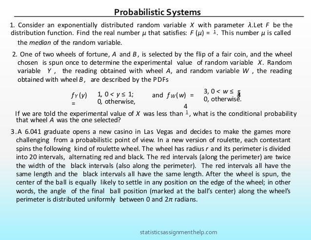
2. One of two wheels of fortune, A and B, is selected by the flip of a fair coin, and the wheel
chosen is spun once to determine the experimental value of random variable X. Random
variable Y , the reading obtained with wheel A, and random variable W , the reading
obtained with wheel B, are described by the PDFs
fY (y)
=
1, 0 < y ≤ 1;
0, otherwise,
and fW (w) = 1
3
3, 0 < w ≤ ;
0, otherwise.
4
If we are told the experimental value of X was less than 1 , what is the conditional probability
that wheel A was the one selected?
3.A 6.041 graduate opens a new casino in Las Vegas and decides to make the games more
challenging from a probabilistic point of view. In a new version of roulette, each contestant
spins the following kind of roulette wheel. The wheel has radius r and its perimeter is divided
into 20 intervals, alternating red and black. The red intervals (along the perimeter) are twice
the width of the black intervals (also along the perimeter). The red intervals all have the
same length and the black intervals all have the same length. After the wheel is spun, the
center of the ball is equally likely to settle in any position on the edge of the wheel; in other
words, the angle of the final ball position (marked at the ball’s center) along the wheel’s
perimeter is distributed uniformly between 0 and 2π radians.
Probabilistic Systems
statisticsassignmenthelp.com
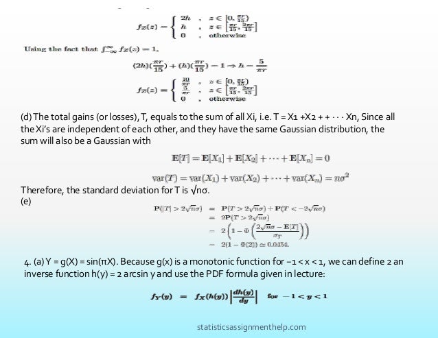
(a)conditional PDF fZ|B(z), where Z is the distance, along the perimeter of the roulette
wheel, between the center of the ball and the edge of the interval immediately clockwise
from the center of the ball?
(b)What is the unconditional PDF fZ (z)?
Another attraction of the casino is the Gaussian slot machine. In this game, the machine
pro- duces independent identically distributed (IID) numbers X1, X2, ... that have normal
distribution N(0, σ2). For every i, when the number Xi is positive, the player receives from
the casino a sum of money equal to Xi. When Xi is negative, the player pays the casino a
sum of money equal to
|Xi|.
(d)What is the standard deviation of the net total gain of a player after n plays of the
Gaussian slot machine?
(e)What is the probability that the absolute value of the net total gain after n plays is
greater than 2√
nσ?
3.Let a continuous random variable X be uniformly distributed over the interval [−1, 1].
Derive the PDF fY (y) where:
(a)What is the probability that the center of the ball settles in a red interval?
(b)Let B denote the event that the center of the ball settles in a black interval. Find
the
statisticsassignmenthelp.com
(a) Y = sin( π X ) 2
(b) Y = sin(2πX)
5 . A Communication Example During lecture, we looked at a simple point-to-point
communi- cation example. The task was to transmit messages from one point to another, by
using a noisy channel. We modeled the problem probabilistically as follows:
• A binary message source generates independent successive messages M1, M2, · · · : each
mes- sage is a discrete random variable that takes the value 1 with probability p and the
value 0 with probability 1 − p. For a single message, we write the PMF as:
pM (m) =1 − p If m = 0
p If m = 1
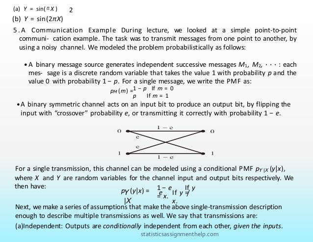
• A binary symmetric channel acts on an input bit to produce an output bit, by flipping the
input with “crossover” probability e, or transmitting it correctly with probability 1 − e.
For a single transmission, this channel can be modeled using a conditional PMF pY |X (y|x),
where X and Y are random variables for the channel input and output bits respectively. We
then have:
Y
|X
p (y|x) = 1 − e If y
= x.
e If y =
/
x.
Next, we make a series of assumptions that make the above single-transmission description
enough to describe multiple transmissions as well. We say that transmissions are:
(a)Independent: Outputs are conditionally independent from each other, given the inputs.
statisticsassignmenthelp.com
(a)Memoryless: Only the current input affects the current output.
(b)Time-invariant: We always have the same conditional PMF.
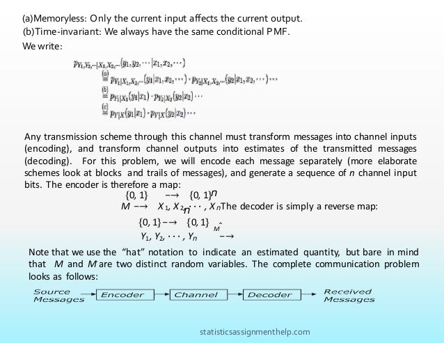
We write:
Any transmission scheme through this channel must transform messages into channel inputs
(encoding), and transform channel outputs into estimates of the transmitted messages
(decoding). For this problem, we will encode each message separately (more elaborate
schemes look at blocks and trails of messages), and generate a sequence of n channel input
bits. The encoder is therefore a map:
{0, 1} −→ {0, 1}n
M −→ X 1, X 2, · · · , X nThe decoder is simply a reverse map:
n
{0, 1}−→ {0, 1}
Y1, Y2, · · · , Yn −→
Mˆ
Note that we use the “hat” notation to indicate an estimated quantity, but bare in mind
that M and Mˆ are two distinct random variables. The complete communication problem
looks as follows:
statisticsassignmenthelp.com
Finally, to measure the performance of any transmission scheme, we look at the probability of
error, i.e. the event that the estimated message is different than the transmitted message:
P(error) = P(M
ˆ /= M ).
M
ˆ (y1, · · · , yn) =
(a)No encoding:
The simplest encoder sends each message bit directly through the channel, i.e. X1 = X
= M . Then, a reasonable decoder is to use the output channel directly as message
estimate: Mˆ= Y1 = Y . What is the probability of error in this case?
(b)Repetition code with majority decoding rule:
The next thing we attempt to do is to send each message n > 1 times through this
channel. On the decoder end, we do what seems natural: decide 0 when there are more
0s than 1s, and decide 1 otherwise. This is a “majority” decoding rule, and we can write
it as follows (making the dependence of Mˆon the channel outputs explicit):
0 If y1 + · · · + yn < n/2.
1 If y1 + · · · + yn ≥ n/2.
Analytical results:
i. Find an expression of the probability of error as a function of e, p and n. [Hint: First
use the total probability rule to divide the problem into solving P(error|M = 0) and
P(error|M = 1), as we did in the lecture.]
ii.Choose p = 0.5, e = 0.3 and use your favorite computational method to make a plot of
P(error) versus n, for n = 1, · · · , 15.
iii.Is majority decoding rule optimal (lowest P(error)) for all p? [Hint: What is the best
decoding rule if p = 0?].
statisticsassignmenthelp.com
Simulation:
i.Set p = 0.5, e = 0.3, generate a message of length 20.
ii.Encode your message with n = 3.
iii.Transmit the message, decode it, and write down the value of the message error rate (the
ratio of bits in error, over the total number of message bits).
iv.Repeat Step 3 serveral times, and average out all the message error rates that you obtain.
How does this compare to your analytical expression of P(error) for this value of n?
v.Repeat Steps 3 and 4 for n = 5, 10, 15, and compare the respective average message error
rates to the corresponding analytical P(error).
(c) Repetition code with maximum a posteriori (MAP) rule:
In Part b, majority decoding was chosen almost arbitrarily, and we have alluded to the fact that it
might not be the best choice in some cases. Here, we claim that the probability of error is in fact
minimized when the decoding rule is as follows
This decoding rule is called “maximum a posterior” or MAP, because it chooses the value of
M which maximizes the posterior probability of M given the channel ouput bits Y1 = y1, ·
· · , Yn = yn (another term for Bayes’ rule).
i.Denote by N0 the number of 0s in y1, · · · , yn, and by N1 the number of 1s. Express
the MAP rule as an inequality in terms of N0 and N1, and as a function of e and p.
[Hint: Use Bayes’ rule to decompose the posterior probability. Note that pY1 ,··· ,Yn
(y1, · · · , yn) is a constant during one decoding.]
statisticsassignmenthelp.com
i. Show that the MAP rule reduces to the majority rule if p = 0.5.
ii. Give an interpretation of how, for p /= 0.5, the MAP rule deviates from the majority
rule. [Hint: Use the simplification steps of your previous answer, but keep p
arbitrary.]
iii.(Optional) Prove that the MAP rule minimizes P(error).
G1†. Let X1, X2, . . . , Xn, . . . be a sequence of independent and identically distributed random
variables. We define random variables S1, S2, . . . , Sn, . . . (n = 1, 2 . . .) in the following
manner: Sn = X1 + X2 + · · · + Xn. Find
E [X 1 | Sn = sn,Sn+ 1 = sn+ 1, . . .]
∫ µ −λ
x
1
λe dx =
2
2
1. We are given that F (µ) = 1
⇒
⇒
1
−λx −λx µ −λµ
λe dx = −e |0 = 1 −e = 2
∫0
µ
0
1
⇒ −λµ = ln 2
ln 2
⇒ µ
=
λ
2. First we can draw a tree with the the following branches:
1
1
fY (y)
1/4
f W (w)
Y>1/4
A
B
Y<1/4
W>1/4
W<1/4
y
3
w
statisticsassignmenthelp.com
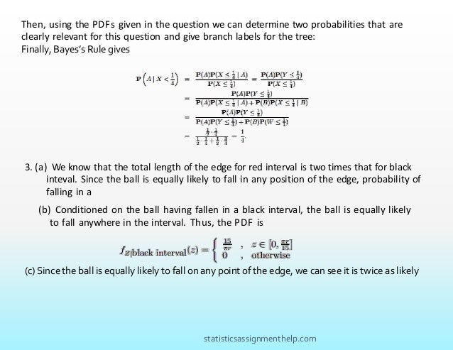
Then, using the PDFs given in the question we can determine two probabilities that are
clearly relevant for this question and give branch labels for the tree:
Finally, Bayes’s Rule gives
3. (a) We know that the total length of the edge for red interval is two times that for black
inteval. Since the ball is equally likely to fall in any position of the edge, probability of
falling in a
(b) Conditioned on the ball having fallen in a black interval, the ball is equally likely
to fall anywhere in the interval. Thus, the PDF is
(c) Since the ball is equally likely to fall on any point of the edge, we can see it is twice as likely
statisticsassignmenthelp.com
(d)The total gains (or losses),T, equals to the sum of all Xi, i.e.T = X1 +X2 + + · · · Xn, Since all
the Xi’s are independent of each other, and they have the same Gaussian distribution, the
sum will also be a Gaussian with
Therefore, the standard deviation forT is √nσ.
(e)
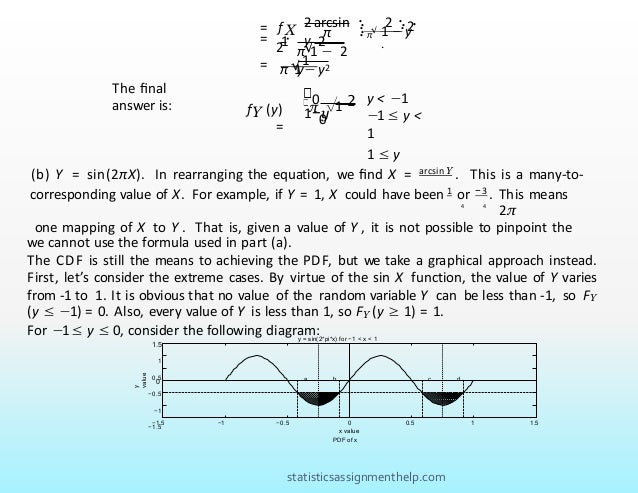
4. (a)Y = g(X) = sin(πX). Because g(x) is a monotonic function for −1 < x < 1, we can define 2 an
inverse function h(y) = 2 arcsin y and use the PDF formula given in lecture:
statisticsassignmenthelp.com
. .
= √
2
. .
2 arcsin
y
= f X .
. √ . .
2
1 −y
.
π . π
1 2
= ·
2 2
√
π 1 −
y
1
π 1 −y2
The final
answer is: 0 y < −1
−1 ≤ y <
1
1 ≤ y
Y
f (y)
=
√1 2
π
1−y
0
(b) Y = sin(2πX). In rearranging the equation, we find X = arcsin Y . This is a many-to-
2π
one mapping of X to Y . That is, given a value of Y , it is not possible to pinpoint the
corresponding value of X. For example, if Y = 1, X could have been 1 or −3 . This means
4 4
we cannot use the formula used in part (a).
The CDF is still the means to achieving the PDF, but we take a graphical approach instead.
First, let’s consider the extreme cases. By virtue of the sin X function, the value of Y varies
from -1 to 1. It is obvious that no value of the random variable Y can be less than -1, so FY
(y ≤ −1) = 0. Also, every value of Y is less than 1, so FY (y ≥ 1) = 1.
For −1≤ y ≤ 0, consider the following diagram:
y = sin(2*pi*x) for −1 < x < 1
y
value
1.5
1
0.5
0
−0.5
−1
−1.5
−1.5 −1 −0.5 0
x value
0.5 1 1.5
a b c d
PDF of x
statisticsassignmenthelp.com
PDF of x
−0.2
0
0.6
0.4
0.2
d
a b c
f(x)
−1.5 −1 −0.5 0
x
0.5 1 1.5
π
π
The value b indicates the conventional response of arcsin
y which is between [
2
2
— , ].
In
other words, by rearranging the
original equation:
b = arcsin y
2
π
1 1
4
4
— ≤
b ≤
So, we now have FY (y) = P((a ≤ X ≤ b) ∪ (c ≤ X ≤ d)), where the event on the
right is the shaded region in the above PDF of X. By symmetry, and mutual exclusivity,
this shaded region can be expressed as four times the more darkly shaded region of
the PDF.
1
FY (y| − 1 ≤ y ≤ 0) = P((a ≤ X ≤
b) ∪ (c ≤ X ≤ d))
=
4P −4
≤ X
≤ b
1
= 4(0.5) b −
−4
arcsin y
1
= + .
π 2
statisticsassignmenthelp.com
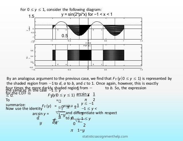
For 0 ≤ y ≤ 1, consider the following diagram:
y = sin(2*pi*x) for −1 < x < 1
1.5
1
0.5
f(x
)
y
value 0
−0.5
−1
−1.5
−1.5 −1 −0.5 0.5 1 1.5
d a b c
0
x value
PDF of x
0.6
0.4
0.2
0
−0.2
a
d b c
−1.5 −1 −0.5 0.5 1 1.5
0
x
By an analogous argument to the previous case, we find that FY (y|0 ≤ y ≤ 1) is represented by
the shaded region from −1to d, a to b, and c to 1. Once again, however, this is exactly
1
four times the more darkly shaded region from − to b. So, the expression
for the CDF is
the same as in the case −1 ≤ y
≤ 0. Y 0 ≤ y ≤ 1)
=
F (y| +
arcsin y 1
π 2
To
summarize: 0arcsin y + 1 y ≤ −1
−1 ≤ y <
1
1 ≤ y
FY (y) = π 2
1
1
d
Now use the identity
arcsin y = √ and differentiate with respect
to y:
1−y
2 0
d
y Y
√1
dy
2
π 1−y
0
statisticsassignmenthelp.com
= P(atleast (m + 1) errors|M = 0)(1 −p) + P(atleast (m + 1) errors|M
= 0)p
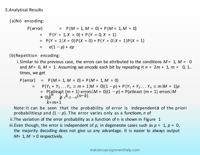
5.Analytical Results
(a)No encoding:
P(error) = P(M
ˆ = 1, M = 0) + P (M
ˆ = 1, M = 0)
= P(Y = 1, X = 0) + P(Y = 0, X = 1)
= P(Y = 1|X = 0)P(X = 0) + P(Y = 0|X = 1)P(X = 1)
= e(1 −p) + ep
(b)Repetition encoding:
i.Similar to the previous case, the errors can be attributed to the conditions Mˆ = 1, M = 0
and Mˆ= 0, M = 1. Assuming we encode each bit by repeating it n = 2m + 1, m = 0, 1..
times, we get
P (error) = P(M
ˆ = 1, M = 0) + P(M
ˆ = 1, M = 0)
= P(Y1 + Y2 . . . Yn ≥ m + 1|M = 0)(1 −p) + P(Y1 + Y2 . . . Yn ≤ m|M = 1)p
Σn !
n ek (1 −e)(n−k)
= k
k=m+1
Note: It can be seen that the probability of error is independenta of the priori
probabilitiesp and (1 −p). The error varies only as a functioen, n of
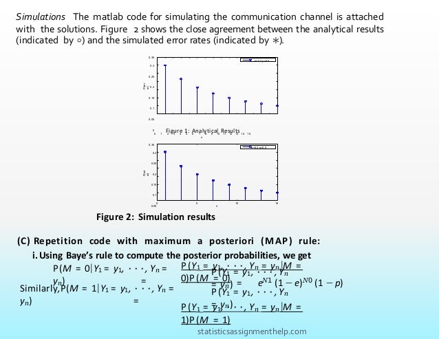
ii.The variation of the error probability as a function of n is shown in Figure 1
iii.Even though, the error is independent of p, in degenerate cases such as p = 1, p = 0,
the majority decoding does not give us any advantage. It is easier to always output
Mˆ= 1, M ˆ= 0 respectively.
statisticsassignmenthelp.com
Simulations The matlab code for simulating the communication channel is attached
with the solutions. Figure 2 shows the close agreement between the analytical results
(indicated by ◦) and the simulated error rates (indicated by ∗).
0.35
0.3
0.25
0.2
0.15
0.1
0.05
0
0 1 2 3 4 5 6 7 8 9 10 11 12 13 14 15
n
P(err
or)
P(err
or)
e=0.3,p=0.5
Figure 1: Analytical Results
0.35
0.3
0.25
0.2
0.15
0.1
0.05
0
0 5 10 15
n
e=0.3,p=0.5
Figure 2: Simulation results
(C) Repetition code with maximum a posteriori (MAP) rule:
i.Using Baye’s rule to compute the posterior probabilities, we get
P(Y1 = y1, ···, Yn = yn|M =
0)P(M = 0)
P(M = 0|Y1 = y1, ···, Yn =
yn) =
P(Y1 = y1, ···, Yn
= yn) = eN1 (1 −e)N0 (1 −p)
P(Y1 = y1, ···, Yn = yn|M =
1)P(M = 1)
Similarly,P(M = 1|Y1 = y1, ···, Yn =
yn) =
P(Y1 = y1, ···, Yn
= yn)
statisticsassignmenthelp.com
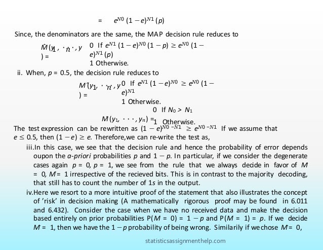
ii. When, p = 0.5, the decision rule reduces to
The test expression can be rewritten as (1 − e)N0 −N1 ≥ eN0 −N1 If we assume that
e ≤ 0.5, then (1 −e) ≥ e. Therefore,we can re-write the test as,
ˆ 1 n
M (y , ···, y
) =
0 If eN1 (1 − e)N0 ≥ eN0 (1 −
e)N1
1 Otherwise.
M
ˆ (y1, ···, yn) =
0 If N0 > N1
1 Otherwise.
iii.In this case, we see that the decision rule and hence the probability of error depends
oupon the a-priori probabilities p and 1 − p. In particular, if we consider the degenerate
cases again p = 0, p = 1, we see from the rule that we always decide in favor of Mˆ
= 0, Mˆ= 1 irrespective of the recieved bits. This is in contrast to the majority decoding,
that still has to count the number of 1s in the output.
iv.Here we resort to a more intuitive proof of the statement that also illustrates the concept
of ’risk’ in decision making (A mathematically rigorous proof may be found in 6.011
and 6.432). Consider the case when we have no received data and make the decision
based entirely on prior probabilities P(M = 0) = 1 − p and P(M = 1) = p. If we decide
Mˆ = 1, then we have the 1 −p probability of being wrong. Similarily if we chose Mˆ= 0,
= eN0 (1 −e)N1 (p)
Since, the denominators are the same, the MAP decision rule reduces to
ˆ 1 n
M (y , ···, y
) =
0 If eN1 (1 − e)N0 (1 −p) ≥ eN0 (1 −
e)N1 (p)
1 Otherwise.
statisticsassignmenthelp.com
M̂ = arg max P (X = M )
M =(0,1)
When we are given the data Y , we have to deal with the a-posteriori probabilities
P(M = 1|Y ), P(M = 0|Y ) instead of a-priori probabilities P(M = 0), P(M = 1) and the
argument remains unchanged. Thus, to minimize probability or being wrong, or
maximize the probability of being right,we choose
M̂ = arg max P (X = M |Y )
M =(0,1)
G1†. Note that we can rewrite E[X1 | Sn = sn,Sn+1 = sn+1, . . .] as follows:
E [X 1 | Sn = sn,Sn+ 1 = sn+ 1, . . .]
= E [X 1 | Sn = sn,X n+ 1 = sn+ 1 − sn,X n+ 2 = sn+ 2 −sn+ 1, . . .]
= E [X 1 | Sn = sn],
where the last equality holds due to the fact that the Xi’s are independent. We
also note that
E [X 1 + ···+ X n | Sn = sn] = E [Sn | Sn = sn] = sn
It follows from the linearity of expectations that
E [X 1 + ···+ X n | Sn = sn] = E [X 1 | Sn = sn] + ···+ E [X n | Sn = sn]/
iii.we have a probability p of being wrong. We choose Mˆto minimize the risk of being
wrong or maximize the probability of being right. Thus we choose
statisticsassignmenthelp.com
Because the Xi’s are identically distributed, we have the following relationship:
E [X i | Sn = sn] = E [X j | Sn = sn], for any 1 ≤ i ≤ n, 1 ≤ j ≤ n.
Therefore,
sn
1 n n
E [X 1 + ···+ X n | Sn = sn] = nE [X 1 | Sn = sn] = sn ⇒ E [X | S = s ]
=
.
n
statisticsassignmenthelp.com

Probabilistic systems assignment help

  • 1.
    For any helpregarding Stochastic Processes Assignment Help Visit :- https://www.statisticsassignmenthelp.com/ , Email :- info@statisticsassignmenthelp.com or Call us at :- +1 678 648 4277 Probabilistic Systems Assignment Help
  • 2.
    1. Consider anexponentially distributed random variable X with parameter λ.Let F be the distribution function. Find the real number µ that satisfies: F (µ) = 1 . This number µ is called the median of the random variable. 2. One of two wheels of fortune, A and B, is selected by the flip of a fair coin, and the wheel chosen is spun once to determine the experimental value of random variable X. Random variable Y , the reading obtained with wheel A, and random variable W , the reading obtained with wheel B, are described by the PDFs fY (y) = 1, 0 < y ≤ 1; 0, otherwise, and fW (w) = 1 3 3, 0 < w ≤ ; 0, otherwise. 4 If we are told the experimental value of X was less than 1 , what is the conditional probability that wheel A was the one selected? 3.A 6.041 graduate opens a new casino in Las Vegas and decides to make the games more challenging from a probabilistic point of view. In a new version of roulette, each contestant spins the following kind of roulette wheel. The wheel has radius r and its perimeter is divided into 20 intervals, alternating red and black. The red intervals (along the perimeter) are twice the width of the black intervals (also along the perimeter). The red intervals all have the same length and the black intervals all have the same length. After the wheel is spun, the center of the ball is equally likely to settle in any position on the edge of the wheel; in other words, the angle of the final ball position (marked at the ball’s center) along the wheel’s perimeter is distributed uniformly between 0 and 2π radians. Probabilistic Systems statisticsassignmenthelp.com
  • 3.
    (a)conditional PDF fZ|B(z),where Z is the distance, along the perimeter of the roulette wheel, between the center of the ball and the edge of the interval immediately clockwise from the center of the ball? (b)What is the unconditional PDF fZ (z)? Another attraction of the casino is the Gaussian slot machine. In this game, the machine pro- duces independent identically distributed (IID) numbers X1, X2, ... that have normal distribution N(0, σ2). For every i, when the number Xi is positive, the player receives from the casino a sum of money equal to Xi. When Xi is negative, the player pays the casino a sum of money equal to |Xi|. (d)What is the standard deviation of the net total gain of a player after n plays of the Gaussian slot machine? (e)What is the probability that the absolute value of the net total gain after n plays is greater than 2√ nσ? 3.Let a continuous random variable X be uniformly distributed over the interval [−1, 1]. Derive the PDF fY (y) where: (a)What is the probability that the center of the ball settles in a red interval? (b)Let B denote the event that the center of the ball settles in a black interval. Find the statisticsassignmenthelp.com
  • 4.
    (a) Y =sin( π X ) 2 (b) Y = sin(2πX) 5 . A Communication Example During lecture, we looked at a simple point-to-point communi- cation example. The task was to transmit messages from one point to another, by using a noisy channel. We modeled the problem probabilistically as follows: • A binary message source generates independent successive messages M1, M2, · · · : each mes- sage is a discrete random variable that takes the value 1 with probability p and the value 0 with probability 1 − p. For a single message, we write the PMF as: pM (m) =1 − p If m = 0 p If m = 1 • A binary symmetric channel acts on an input bit to produce an output bit, by flipping the input with “crossover” probability e, or transmitting it correctly with probability 1 − e. For a single transmission, this channel can be modeled using a conditional PMF pY |X (y|x), where X and Y are random variables for the channel input and output bits respectively. We then have: Y |X p (y|x) = 1 − e If y = x. e If y = / x. Next, we make a series of assumptions that make the above single-transmission description enough to describe multiple transmissions as well. We say that transmissions are: (a)Independent: Outputs are conditionally independent from each other, given the inputs. statisticsassignmenthelp.com
  • 5.
    (a)Memoryless: Only thecurrent input affects the current output. (b)Time-invariant: We always have the same conditional PMF. We write: Any transmission scheme through this channel must transform messages into channel inputs (encoding), and transform channel outputs into estimates of the transmitted messages (decoding). For this problem, we will encode each message separately (more elaborate schemes look at blocks and trails of messages), and generate a sequence of n channel input bits. The encoder is therefore a map: {0, 1} −→ {0, 1}n M −→ X 1, X 2, · · · , X nThe decoder is simply a reverse map: n {0, 1}−→ {0, 1} Y1, Y2, · · · , Yn −→ Mˆ Note that we use the “hat” notation to indicate an estimated quantity, but bare in mind that M and Mˆ are two distinct random variables. The complete communication problem looks as follows: statisticsassignmenthelp.com
  • 6.
    Finally, to measurethe performance of any transmission scheme, we look at the probability of error, i.e. the event that the estimated message is different than the transmitted message: P(error) = P(M ˆ /= M ). M ˆ (y1, · · · , yn) = (a)No encoding: The simplest encoder sends each message bit directly through the channel, i.e. X1 = X = M . Then, a reasonable decoder is to use the output channel directly as message estimate: Mˆ= Y1 = Y . What is the probability of error in this case? (b)Repetition code with majority decoding rule: The next thing we attempt to do is to send each message n > 1 times through this channel. On the decoder end, we do what seems natural: decide 0 when there are more 0s than 1s, and decide 1 otherwise. This is a “majority” decoding rule, and we can write it as follows (making the dependence of Mˆon the channel outputs explicit): 0 If y1 + · · · + yn < n/2. 1 If y1 + · · · + yn ≥ n/2. Analytical results: i. Find an expression of the probability of error as a function of e, p and n. [Hint: First use the total probability rule to divide the problem into solving P(error|M = 0) and P(error|M = 1), as we did in the lecture.] ii.Choose p = 0.5, e = 0.3 and use your favorite computational method to make a plot of P(error) versus n, for n = 1, · · · , 15. iii.Is majority decoding rule optimal (lowest P(error)) for all p? [Hint: What is the best decoding rule if p = 0?]. statisticsassignmenthelp.com
  • 7.
    Simulation: i.Set p =0.5, e = 0.3, generate a message of length 20. ii.Encode your message with n = 3. iii.Transmit the message, decode it, and write down the value of the message error rate (the ratio of bits in error, over the total number of message bits). iv.Repeat Step 3 serveral times, and average out all the message error rates that you obtain. How does this compare to your analytical expression of P(error) for this value of n? v.Repeat Steps 3 and 4 for n = 5, 10, 15, and compare the respective average message error rates to the corresponding analytical P(error). (c) Repetition code with maximum a posteriori (MAP) rule: In Part b, majority decoding was chosen almost arbitrarily, and we have alluded to the fact that it might not be the best choice in some cases. Here, we claim that the probability of error is in fact minimized when the decoding rule is as follows This decoding rule is called “maximum a posterior” or MAP, because it chooses the value of M which maximizes the posterior probability of M given the channel ouput bits Y1 = y1, · · · , Yn = yn (another term for Bayes’ rule). i.Denote by N0 the number of 0s in y1, · · · , yn, and by N1 the number of 1s. Express the MAP rule as an inequality in terms of N0 and N1, and as a function of e and p. [Hint: Use Bayes’ rule to decompose the posterior probability. Note that pY1 ,··· ,Yn (y1, · · · , yn) is a constant during one decoding.] statisticsassignmenthelp.com
  • 8.
    i. Show thatthe MAP rule reduces to the majority rule if p = 0.5. ii. Give an interpretation of how, for p /= 0.5, the MAP rule deviates from the majority rule. [Hint: Use the simplification steps of your previous answer, but keep p arbitrary.] iii.(Optional) Prove that the MAP rule minimizes P(error). G1†. Let X1, X2, . . . , Xn, . . . be a sequence of independent and identically distributed random variables. We define random variables S1, S2, . . . , Sn, . . . (n = 1, 2 . . .) in the following manner: Sn = X1 + X2 + · · · + Xn. Find E [X 1 | Sn = sn,Sn+ 1 = sn+ 1, . . .] ∫ µ −λ x 1 λe dx = 2 2 1. We are given that F (µ) = 1 ⇒ ⇒ 1 −λx −λx µ −λµ λe dx = −e |0 = 1 −e = 2 ∫0 µ 0 1 ⇒ −λµ = ln 2 ln 2 ⇒ µ = λ 2. First we can draw a tree with the the following branches: 1 1 fY (y) 1/4 f W (w) Y>1/4 A B Y<1/4 W>1/4 W<1/4 y 3 w statisticsassignmenthelp.com
  • 9.
    Then, using thePDFs given in the question we can determine two probabilities that are clearly relevant for this question and give branch labels for the tree: Finally, Bayes’s Rule gives 3. (a) We know that the total length of the edge for red interval is two times that for black inteval. Since the ball is equally likely to fall in any position of the edge, probability of falling in a (b) Conditioned on the ball having fallen in a black interval, the ball is equally likely to fall anywhere in the interval. Thus, the PDF is (c) Since the ball is equally likely to fall on any point of the edge, we can see it is twice as likely statisticsassignmenthelp.com
  • 10.
    (d)The total gains(or losses),T, equals to the sum of all Xi, i.e.T = X1 +X2 + + · · · Xn, Since all the Xi’s are independent of each other, and they have the same Gaussian distribution, the sum will also be a Gaussian with Therefore, the standard deviation forT is √nσ. (e) 4. (a)Y = g(X) = sin(πX). Because g(x) is a monotonic function for −1 < x < 1, we can define 2 an inverse function h(y) = 2 arcsin y and use the PDF formula given in lecture: statisticsassignmenthelp.com
  • 11.
    . . = √ 2 .. 2 arcsin y = f X . . √ . . 2 1 −y . π . π 1 2 = · 2 2 √ π 1 − y 1 π 1 −y2 The final answer is: 0 y < −1 −1 ≤ y < 1 1 ≤ y Y f (y) = √1 2 π 1−y 0 (b) Y = sin(2πX). In rearranging the equation, we find X = arcsin Y . This is a many-to- 2π one mapping of X to Y . That is, given a value of Y , it is not possible to pinpoint the corresponding value of X. For example, if Y = 1, X could have been 1 or −3 . This means 4 4 we cannot use the formula used in part (a). The CDF is still the means to achieving the PDF, but we take a graphical approach instead. First, let’s consider the extreme cases. By virtue of the sin X function, the value of Y varies from -1 to 1. It is obvious that no value of the random variable Y can be less than -1, so FY (y ≤ −1) = 0. Also, every value of Y is less than 1, so FY (y ≥ 1) = 1. For −1≤ y ≤ 0, consider the following diagram: y = sin(2*pi*x) for −1 < x < 1 y value 1.5 1 0.5 0 −0.5 −1 −1.5 −1.5 −1 −0.5 0 x value 0.5 1 1.5 a b c d PDF of x statisticsassignmenthelp.com
  • 12.
    PDF of x −0.2 0 0.6 0.4 0.2 d ab c f(x) −1.5 −1 −0.5 0 x 0.5 1 1.5 π π The value b indicates the conventional response of arcsin y which is between [ 2 2 — , ]. In other words, by rearranging the original equation: b = arcsin y 2 π 1 1 4 4 — ≤ b ≤ So, we now have FY (y) = P((a ≤ X ≤ b) ∪ (c ≤ X ≤ d)), where the event on the right is the shaded region in the above PDF of X. By symmetry, and mutual exclusivity, this shaded region can be expressed as four times the more darkly shaded region of the PDF. 1 FY (y| − 1 ≤ y ≤ 0) = P((a ≤ X ≤ b) ∪ (c ≤ X ≤ d)) = 4P −4 ≤ X ≤ b 1 = 4(0.5) b − −4 arcsin y 1 = + . π 2 statisticsassignmenthelp.com
  • 13.
    For 0 ≤y ≤ 1, consider the following diagram: y = sin(2*pi*x) for −1 < x < 1 1.5 1 0.5 f(x ) y value 0 −0.5 −1 −1.5 −1.5 −1 −0.5 0.5 1 1.5 d a b c 0 x value PDF of x 0.6 0.4 0.2 0 −0.2 a d b c −1.5 −1 −0.5 0.5 1 1.5 0 x By an analogous argument to the previous case, we find that FY (y|0 ≤ y ≤ 1) is represented by the shaded region from −1to d, a to b, and c to 1. Once again, however, this is exactly 1 four times the more darkly shaded region from − to b. So, the expression for the CDF is the same as in the case −1 ≤ y ≤ 0. Y 0 ≤ y ≤ 1) = F (y| + arcsin y 1 π 2 To summarize: 0arcsin y + 1 y ≤ −1 −1 ≤ y < 1 1 ≤ y FY (y) = π 2 1 1 d Now use the identity arcsin y = √ and differentiate with respect to y: 1−y 2 0 d y Y √1 dy 2 π 1−y 0 statisticsassignmenthelp.com
  • 14.
    = P(atleast (m+ 1) errors|M = 0)(1 −p) + P(atleast (m + 1) errors|M = 0)p 5.Analytical Results (a)No encoding: P(error) = P(M ˆ = 1, M = 0) + P (M ˆ = 1, M = 0) = P(Y = 1, X = 0) + P(Y = 0, X = 1) = P(Y = 1|X = 0)P(X = 0) + P(Y = 0|X = 1)P(X = 1) = e(1 −p) + ep (b)Repetition encoding: i.Similar to the previous case, the errors can be attributed to the conditions Mˆ = 1, M = 0 and Mˆ= 0, M = 1. Assuming we encode each bit by repeating it n = 2m + 1, m = 0, 1.. times, we get P (error) = P(M ˆ = 1, M = 0) + P(M ˆ = 1, M = 0) = P(Y1 + Y2 . . . Yn ≥ m + 1|M = 0)(1 −p) + P(Y1 + Y2 . . . Yn ≤ m|M = 1)p Σn ! n ek (1 −e)(n−k) = k k=m+1 Note: It can be seen that the probability of error is independenta of the priori probabilitiesp and (1 −p). The error varies only as a functioen, n of ii.The variation of the error probability as a function of n is shown in Figure 1 iii.Even though, the error is independent of p, in degenerate cases such as p = 1, p = 0, the majority decoding does not give us any advantage. It is easier to always output Mˆ= 1, M ˆ= 0 respectively. statisticsassignmenthelp.com
  • 15.
    Simulations The matlabcode for simulating the communication channel is attached with the solutions. Figure 2 shows the close agreement between the analytical results (indicated by ◦) and the simulated error rates (indicated by ∗). 0.35 0.3 0.25 0.2 0.15 0.1 0.05 0 0 1 2 3 4 5 6 7 8 9 10 11 12 13 14 15 n P(err or) P(err or) e=0.3,p=0.5 Figure 1: Analytical Results 0.35 0.3 0.25 0.2 0.15 0.1 0.05 0 0 5 10 15 n e=0.3,p=0.5 Figure 2: Simulation results (C) Repetition code with maximum a posteriori (MAP) rule: i.Using Baye’s rule to compute the posterior probabilities, we get P(Y1 = y1, ···, Yn = yn|M = 0)P(M = 0) P(M = 0|Y1 = y1, ···, Yn = yn) = P(Y1 = y1, ···, Yn = yn) = eN1 (1 −e)N0 (1 −p) P(Y1 = y1, ···, Yn = yn|M = 1)P(M = 1) Similarly,P(M = 1|Y1 = y1, ···, Yn = yn) = P(Y1 = y1, ···, Yn = yn) statisticsassignmenthelp.com
  • 16.
    ii. When, p= 0.5, the decision rule reduces to The test expression can be rewritten as (1 − e)N0 −N1 ≥ eN0 −N1 If we assume that e ≤ 0.5, then (1 −e) ≥ e. Therefore,we can re-write the test as, ˆ 1 n M (y , ···, y ) = 0 If eN1 (1 − e)N0 ≥ eN0 (1 − e)N1 1 Otherwise. M ˆ (y1, ···, yn) = 0 If N0 > N1 1 Otherwise. iii.In this case, we see that the decision rule and hence the probability of error depends oupon the a-priori probabilities p and 1 − p. In particular, if we consider the degenerate cases again p = 0, p = 1, we see from the rule that we always decide in favor of Mˆ = 0, Mˆ= 1 irrespective of the recieved bits. This is in contrast to the majority decoding, that still has to count the number of 1s in the output. iv.Here we resort to a more intuitive proof of the statement that also illustrates the concept of ’risk’ in decision making (A mathematically rigorous proof may be found in 6.011 and 6.432). Consider the case when we have no received data and make the decision based entirely on prior probabilities P(M = 0) = 1 − p and P(M = 1) = p. If we decide Mˆ = 1, then we have the 1 −p probability of being wrong. Similarily if we chose Mˆ= 0, = eN0 (1 −e)N1 (p) Since, the denominators are the same, the MAP decision rule reduces to ˆ 1 n M (y , ···, y ) = 0 If eN1 (1 − e)N0 (1 −p) ≥ eN0 (1 − e)N1 (p) 1 Otherwise. statisticsassignmenthelp.com
  • 17.
    M̂ = argmax P (X = M ) M =(0,1) When we are given the data Y , we have to deal with the a-posteriori probabilities P(M = 1|Y ), P(M = 0|Y ) instead of a-priori probabilities P(M = 0), P(M = 1) and the argument remains unchanged. Thus, to minimize probability or being wrong, or maximize the probability of being right,we choose M̂ = arg max P (X = M |Y ) M =(0,1) G1†. Note that we can rewrite E[X1 | Sn = sn,Sn+1 = sn+1, . . .] as follows: E [X 1 | Sn = sn,Sn+ 1 = sn+ 1, . . .] = E [X 1 | Sn = sn,X n+ 1 = sn+ 1 − sn,X n+ 2 = sn+ 2 −sn+ 1, . . .] = E [X 1 | Sn = sn], where the last equality holds due to the fact that the Xi’s are independent. We also note that E [X 1 + ···+ X n | Sn = sn] = E [Sn | Sn = sn] = sn It follows from the linearity of expectations that E [X 1 + ···+ X n | Sn = sn] = E [X 1 | Sn = sn] + ···+ E [X n | Sn = sn]/ iii.we have a probability p of being wrong. We choose Mˆto minimize the risk of being wrong or maximize the probability of being right. Thus we choose statisticsassignmenthelp.com
  • 18.
    Because the Xi’sare identically distributed, we have the following relationship: E [X i | Sn = sn] = E [X j | Sn = sn], for any 1 ≤ i ≤ n, 1 ≤ j ≤ n. Therefore, sn 1 n n E [X 1 + ···+ X n | Sn = sn] = nE [X 1 | Sn = sn] = sn ⇒ E [X | S = s ] = . n statisticsassignmenthelp.com