MBA Business Statistics Unit 1 Handwritten Notes with Solved Examples | CA Suvidha Chaplot

MBA Business Statistics Unit 1 Handwritten Notes with Solved Examples | CA Suvidha Chaplot

• 1.
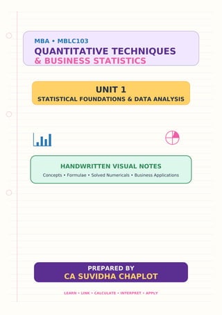
  MBA • MBLC103 QUANTITATIVETECHNIQUES & BUSINESS STATISTICS UNIT 1 STATISTICAL FOUNDATIONS & DATA ANALYSIS HANDWRITTEN VISUAL NOTES Concepts • Formulae • Solved Numericals • Business Applications PREPARED BY CA SUVIDHA CHAPLOT LEARN • LINK • CALCULATE • INTERPRET • APPLY
• 2.
  UNIT 1 |INFOGRAPHIC 02 UNIT 1 ROADMAP Complete syllabus coverage at one glance 1 Nature, Scope & Importance Concept + formula + example + decision use 2 Data Collection & Quality Concept + formula + example + decision use 3 Classification & Presentation Concept + formula + example + decision use 4 Mean, Median & Mode Concept + formula + example + decision use 5 Range, QD, MD, SD & CV Concept + formula + example + decision use 6 Karl Pearson Correlation Concept + formula + example + decision use 7 Spearman Rank Correlation Concept + formula + example + decision use 8 Simple Linear Regression Concept + formula + example + decision use 9 Business Applications Concept + formula + example + decision use EXAM READY: DEFINITIONS + WORKING STEPS + INTERPRETATION CA SUVIDHA CHAPLOT MBLC103 • PAGE 2
• 3.
  UNIT 1 |INFOGRAPHIC 03 STATISTICS: THE BUSINESS COMPASS Meaning • nature • scope • importance What is Statistics? In the plural sense: numerical facts. In the singular sense: the science of collecting, classifying, presenting, analysing and interpreting data for decisions. Why managers need it It converts raw facts into information, compares performance, measures risk, forecasts demand and supports evidence-based decisions. Key features Aggregate of facts • numerically expressed • affected by many causes • collected systematically • for a predetermined purpose • comparable and related. Remember! Statistics does not replace managerial judgment; it sharpens judgment. A result is useful only when the data and method are appropriate. QUICK RECALL → WRITE FORMULA → SHOW WORKING → INTERPRET CA SUVIDHA CHAPLOT MBLC103 • PAGE 3
• 4.
  UNIT 1 |INFOGRAPHIC 04 NATURE, SCOPE & LIMITATIONS See both the power and boundaries of statistics Nature Both a science (systematic principles) and an art (skillful application). It studies groups, not isolated cases, and usually works with quantitative data. Scope Planning • marketing • finance • HR • production • economics • government • research • quality control • banking and insurance. Limitations Studies aggregates; qualitative facts require measurement; results are approximate; association is not always causation; can be misused; needs homogeneous data. Golden rule Define the objective first. Then choose the population, variables, units, time period, sources and suitable statistical tools. QUICK RECALL → WRITE FORMULA → SHOW WORKING → INTERPRET CA SUVIDHA CHAPLOT MBLC103 • PAGE 4
• 5.
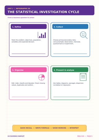
  UNIT 1 |INFOGRAPHIC 05 THE STATISTICAL INVESTIGATION CYCLE From a business question to action 1. Define State the problem, objectives, population, variables and expected decision. 2. Collect Choose primary/secondary data; census/sample; observation, interview, questionnaire or experiment. 3. Organise Edit, code, classify and tabulate. Check missing values, duplicates and outliers. 4. Present & analyse Use tables, diagrams, averages, dispersion, correlation or regression. QUICK RECALL → WRITE FORMULA → SHOW WORKING → INTERPRET CA SUVIDHA CHAPLOT MBLC103 • PAGE 5
• 6.
  UNIT 1 |INFOGRAPHIC 06 DATA: TYPES & SOURCES Build the right foundation before calculation Primary data Collected first-hand for the current objective: survey, interview, observation, schedule, experiment. Specific but costly and time-consuming. Secondary data Already collected: company records, government reports, journals, websites and databases. Quick and economical; verify suitability and reliability. Classification Qualitative/quantitative • discrete/continuous • cross-sectional/time-series • nominal/ordinal/interval/ratio. Quality checklist Relevance • accuracy • adequacy • timeliness • consistency • unbiased source • clearly defined units. QUICK RECALL → WRITE FORMULA → SHOW WORKING → INTERPRET CA SUVIDHA CHAPLOT MBLC103 • PAGE 6
• 7.
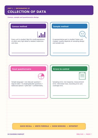
  UNIT 1 |INFOGRAPHIC 07 COLLECTION OF DATA Census, sample and questionnaire design Census method Every unit is studied. Best for small populations or when very high detail is needed; expensive and slow. Sample method A representative part is studied. Faster and cheaper; quality depends on sampling design and sample size. Good questionnaire Simple language • one idea per question • logical order • no leading/double questions • balanced options • pilot test • confidentiality. Errors to control Sampling error, non-response, measurement error, interviewer bias, recording error and coverage error. QUICK RECALL → WRITE FORMULA → SHOW WORKING → INTERPRET CA SUVIDHA CHAPLOT MBLC103 • PAGE 7
• 8.
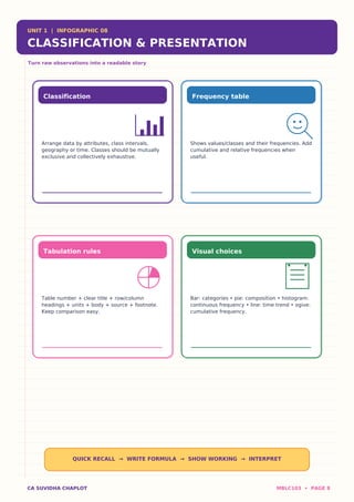
  UNIT 1 |INFOGRAPHIC 08 CLASSIFICATION & PRESENTATION Turn raw observations into a readable story Classification Arrange data by attributes, class intervals, geography or time. Classes should be mutually exclusive and collectively exhaustive. Frequency table Shows values/classes and their frequencies. Add cumulative and relative frequencies when useful. Tabulation rules Table number + clear title + row/column headings + units + body + source + footnote. Keep comparison easy. Visual choices Bar: categories • pie: composition • histogram: continuous frequency • line: time trend • ogive: cumulative frequency. QUICK RECALL → WRITE FORMULA → SHOW WORKING → INTERPRET CA SUVIDHA CHAPLOT MBLC103 • PAGE 8
• 9.
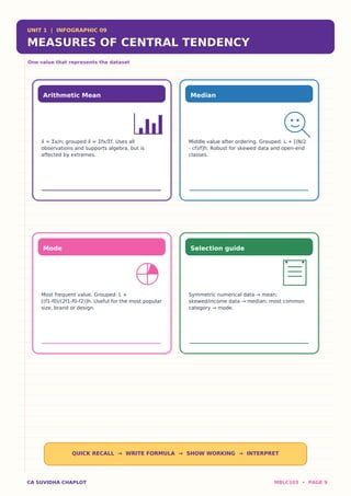
  UNIT 1 |INFOGRAPHIC 09 MEASURES OF CENTRAL TENDENCY One value that represents the dataset Arithmetic Mean x̄ = Σx/n; grouped x̄ = Σfx/Σf. Uses all observations and supports algebra, but is affected by extremes. Median Middle value after ordering. Grouped: L + [(N/2 - cf)/f]h. Robust for skewed data and open-end classes. Mode Most frequent value. Grouped: L + [(f1-f0)/(2f1-f0-f2)]h. Useful for the most popular size, brand or design. Selection guide Symmetric numerical data → mean; skewed/income data → median; most common category → mode. QUICK RECALL → WRITE FORMULA → SHOW WORKING → INTERPRET CA SUVIDHA CHAPLOT MBLC103 • PAGE 9
• 10.
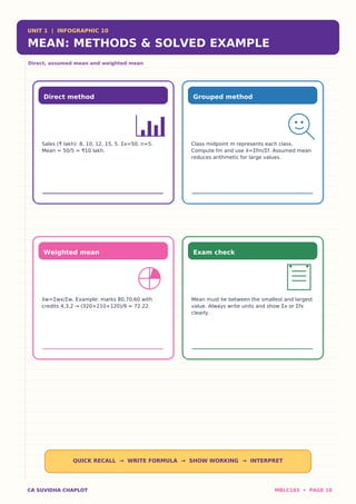
  UNIT 1 |INFOGRAPHIC 10 MEAN: METHODS & SOLVED EXAMPLE Direct, assumed mean and weighted mean Direct method Sales (₹ lakh): 8, 10, 12, 15, 5. Σx=50, n=5. Mean = 50/5 = ₹10 lakh. Grouped method Class midpoint m represents each class. Compute fm and use x̄=Σfm/Σf. Assumed mean reduces arithmetic for large values. Weighted mean x̄w=Σwx/Σw. Example: marks 80,70,60 with credits 4,3,2 → (320+210+120)/9 = 72.22. Exam check Mean must lie between the smallest and largest value. Always write units and show Σx or Σfx clearly. QUICK RECALL → WRITE FORMULA → SHOW WORKING → INTERPRET CA SUVIDHA CHAPLOT MBLC103 • PAGE 10
• 11.
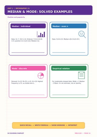
  UNIT 1 |INFOGRAPHIC 11 MEDIAN & MODE: SOLVED EXAMPLES Position and popularity Median - individual Data: 12, 7, 18, 9, 14. Ordered: 7,9,12,14,18. n=5; position=(n+1)/2=3rd. Median=12. Median - even n Data: 5,8,11,15. Median=(8+11)/2=9.5. Mode - discrete Demand: S=12, M=25, L=31, XL=18. Highest frequency is 31, so modal size=L. Empirical relation For moderately skewed data: Mode ≈ 3 Median - 2 Mean. It is an estimate, not an identity. QUICK RECALL → WRITE FORMULA → SHOW WORKING → INTERPRET CA SUVIDHA CHAPLOT MBLC103 • PAGE 11
• 12.
  UNIT 1 |INFOGRAPHIC 12 MEASURES OF DISPERSION Average alone never tells the whole story Meaning Dispersion shows how far observations spread around a central value. Lower dispersion usually means greater consistency. Absolute measures Range, quartile deviation, mean deviation and standard deviation are expressed in the original unit. Relative measures Coefficients and coefficient of variation are unit-free; useful for comparing series with different averages. Business value Compare risk, consistency, wage inequality, demand fluctuation, delivery reliability and quality variation. QUICK RECALL → WRITE FORMULA → SHOW WORKING → INTERPRET CA SUVIDHA CHAPLOT MBLC103 • PAGE 12
• 13.
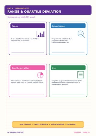
  UNIT 1 |INFOGRAPHIC 13 RANGE & QUARTILE DEVIATION Quick spread and middle-50% spread Range R=L-S. Coefficient=(L-S)/(L+S). Fast but depends only on extremes. Solved range Daily demand: 18,20,21,25,31. Range=31-18=13 units. Coefficient=13/49=0.265. Quartile deviation QD=(Q3-Q1)/2. Coefficient=(Q3-Q1)/(Q3+Q1). Ignores outer 50%, so it resists extreme values. Use Range for rough control/temperature; QD for skewed distributions, open-end classes or median-based reporting. QUICK RECALL → WRITE FORMULA → SHOW WORKING → INTERPRET CA SUVIDHA CHAPLOT MBLC103 • PAGE 13
• 14.
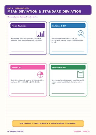
  UNIT 1 |INFOGRAPHIC 14 MEAN DEVIATION & STANDARD DEVIATION Measure typical distance from the centre Mean deviation MD about A = Σ|x-A|/n; grouped = Σf|x-A|/N. Absolute signs prevent deviations cancelling. Variance & SD Population variance σ²=Σ(x-x̄)²/N; SD σ=√variance. Sample variance usually divides by n-1. Solved SD Data 2,4,6. Mean=4; squared deviations=4,0,4; variance=8/3=2.667; SD=√2.667=1.633. Interpretation SD=0 only when all values are equal. Larger SD means greater variability in the same unit as data. QUICK RECALL → WRITE FORMULA → SHOW WORKING → INTERPRET CA SUVIDHA CHAPLOT MBLC103 • PAGE 14
• 15.
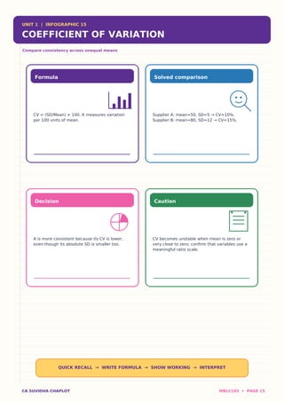
  UNIT 1 |INFOGRAPHIC 15 COEFFICIENT OF VARIATION Compare consistency across unequal means Formula CV = (SD/Mean) × 100. It measures variation per 100 units of mean. Solved comparison Supplier A: mean=50, SD=5 → CV=10%. Supplier B: mean=80, SD=12 → CV=15%. Decision A is more consistent because its CV is lower, even though its absolute SD is smaller too. Caution CV becomes unstable when mean is zero or very close to zero; confirm that variables use a meaningful ratio scale. QUICK RECALL → WRITE FORMULA → SHOW WORKING → INTERPRET CA SUVIDHA CHAPLOT MBLC103 • PAGE 15
• 16.
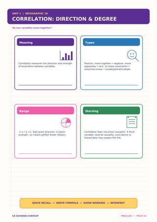
  UNIT 1 |INFOGRAPHIC 16 CORRELATION: DIRECTION & DEGREE Do two variables move together? Meaning Correlation measures the direction and strength of association between variables. Types Positive: move together • negative: move oppositely • zero: no linear association • linear/non-linear • simple/partial/multiple. Range -1 ≤ r ≤ +1. Sign gives direction; |r| gives strength. ±1 means perfect linear relation. Warning Correlation does not prove causation. A third variable, reverse causality, coincidence or biased data may explain the link. QUICK RECALL → WRITE FORMULA → SHOW WORKING → INTERPRET CA SUVIDHA CHAPLOT MBLC103 • PAGE 16
• 17.
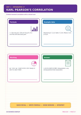
  UNIT 1 |INFOGRAPHIC 17 KARL PEARSON’S CORRELATION Product-moment correlation with a solved case Formula r = Σ[(x-x̄)(y-ȳ)] / √[Σ(x-x̄)² Σ(y-ȳ)²]. It is unit-free and uses every pair. Example data Advertising X: 1,2,3; Sales Y: 2,4,5. Means: x̄=2, ȳ=11/3. Working dx: -1,0,1; dy: -1.667,0.333,1.333. Σdxdy=3; Σdx²=2; Σdy²=4.667. Answer r=3/√(2×4.667)=0.982. Interpretation: very strong positive linear association. QUICK RECALL → WRITE FORMULA → SHOW WORKING → INTERPRET CA SUVIDHA CHAPLOT MBLC103 • PAGE 17
• 18.
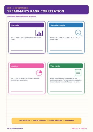
  UNIT 1 |INFOGRAPHIC 18 SPEARMAN’S RANK CORRELATION Association when information is in ranks Formula ρ = 1 - [6Σd² / n(n²-1)] when there are no tied ranks. Solved example Ranks X: 1,2,3,4,5; Y: 2,1,3,5,4. d: -1,1,0,-1,1; Σd²=4; n=5. Answer ρ = 1 - 24/[5×24] = 0.80. There is a strong positive rank association. Tied ranks Assign each tied item the average of the positions occupied. For rigorous work, apply the tie correction or compute Pearson r on ranks. QUICK RECALL → WRITE FORMULA → SHOW WORKING → INTERPRET CA SUVIDHA CHAPLOT MBLC103 • PAGE 18
• 19.
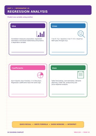
  UNIT 1 |INFOGRAPHIC 19 REGRESSION ANALYSIS Predict one variable using another Idea Correlation measures association; regression estimates a functional relationship and predicts a dependent variable. Lines Y on X: Y-ȳ = byx(X-x̄). X on Y: X-x̄ = bxy(Y-ȳ). Both pass through (x̄,ȳ). Coefficients byx=r(σy/σx); bxy=r(σx/σy); r=±√(bxy·byx). Regression coefficients have the same sign. Uses Sales forecasting, cost estimation, demand planning, credit risk, productivity and price-response analysis. QUICK RECALL → WRITE FORMULA → SHOW WORKING → INTERPRET CA SUVIDHA CHAPLOT MBLC103 • PAGE 19
• 20.
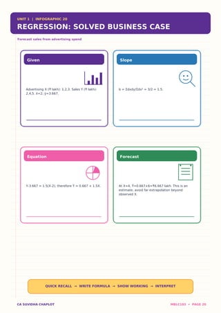
  UNIT 1 |INFOGRAPHIC 20 REGRESSION: SOLVED BUSINESS CASE Forecast sales from advertising spend Given Advertising X (₹ lakh): 1,2,3. Sales Y (₹ lakh): 2,4,5. x̄=2; ȳ=3.667. Slope b = Σdxdy/Σdx² = 3/2 = 1.5. Equation Y-3.667 = 1.5(X-2), therefore Ŷ = 0.667 + 1.5X. Forecast At X=4, Ŷ=0.667+6=₹6.667 lakh. This is an estimate; avoid far extrapolation beyond observed X. QUICK RECALL → WRITE FORMULA → SHOW WORKING → INTERPRET CA SUVIDHA CHAPLOT MBLC103 • PAGE 20
• 21.
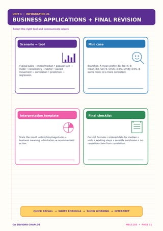
  UNIT 1 |INFOGRAPHIC 21 BUSINESS APPLICATIONS + FINAL REVISION Select the right tool and communicate wisely Scenario → tool Typical sales → mean/median • popular size → mode • consistency → SD/CV • paired movement → correlation • prediction → regression. Mini case Branches: A mean profit=40, SD=4; B mean=60, SD=9. CV(A)=10%, CV(B)=15%. B earns more; A is more consistent. Interpretation template State the result → direction/magnitude → business meaning → limitation → recommended action. Final checklist Correct formula • ordered data for median • units • working steps • sensible conclusion • no causation claim from correlation. QUICK RECALL → WRITE FORMULA → SHOW WORKING → INTERPRET CA SUVIDHA CHAPLOT MBLC103 • PAGE 21