CS 332 - Algorithms Dynamic programming 0-1 Knapsack problem
Review: Dynamic programming DP is a method for solving certain kind of problems DP can be applied when the solution of a problem includes solutions to subproblems We need to find a recursive formula for the solution We can recursively solve subproblems, starting from the trivial case, and save their solutions in memory In the end we’ll get the solution of the whole problem
Properties of a problem that can be solved with dynamic programming Simple Subproblems We should be able to break the original problem to smaller subproblems that have the same structure Optimal Substructure of the problems The solution to the problem must be a composition of subproblem solutions Subproblem Overlap Optimal subproblems to unrelated problems can contain subproblems in common
Review:  Longest Common Subsequence (LCS) Problem: how to find the longest pattern of characters that is common to two text strings X and Y Dynamic programming algorithm: solve subproblems until we get the final solution Subproblem: first find the LCS of  prefixes  of X and Y. this problem has  optimal substructure : LCS of two prefixes is always a part of LCS of bigger strings
Review:  Longest Common Subsequence (LCS) continued Define X i , Y j  to be prefixes of X and Y of length i and j; m = |X|, n = |Y|   We store the length of LCS(X i , Y j ) in c[i,j] Trivial cases: LCS(X 0  , Y j  ) and LCS(X i , Y 0 ) is empty (so c[0,j] = c[i,0] = 0 ) Recursive formula for c[i,j]: c[m,n] is the final solution
Review:  Longest Common Subsequence (LCS) After we have filled the array  c[ ],  we can use this data to find the characters that constitute the Longest Common Subsequence Algorithm runs in  O(m*n) , which is  much  better than the brute-force algorithm:  O(n 2 m )
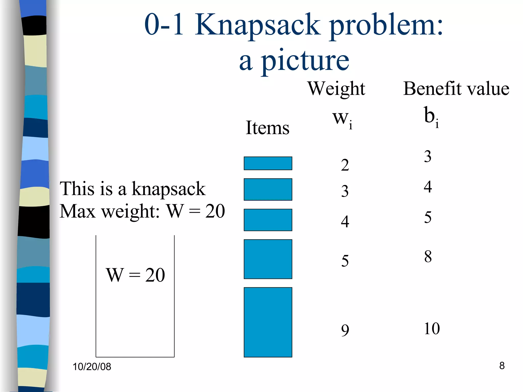
0-1 Knapsack problem Given a knapsack with maximum capacity  W , and a set  S  consisting of  n  items Each item  i  has some weight  w i  and benefit value  b i   (all  w i  , b i   and  W  are integer values) Problem : How to pack the knapsack to achieve maximum total value of packed items?
0-1 Knapsack problem: a picture w i b i 10 9 8 5 5 4 4 3 3 2 Weight Benefit value This is a knapsack Max weight: W = 20 Items W = 20
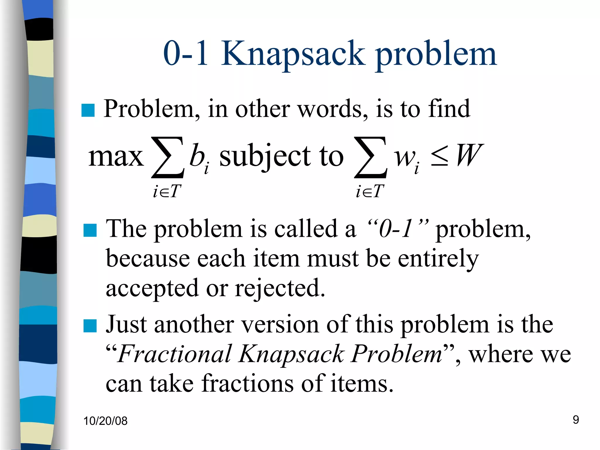
0-1 Knapsack problem Problem, in other words, is to find The problem is called a  “0-1”  problem, because each item must be entirely accepted or rejected. Just another version of this problem is the “ Fractional Knapsack Problem ”, where we can take fractions of items.
0-1 Knapsack problem: brute-force approach Let’s first solve this problem with a straightforward algorithm Since there are  n  items, there are  2 n  possible combinations of items. We go through all combinations and find the one with the most total value and with total weight less or equal to  W Running time will be  O(2 n )
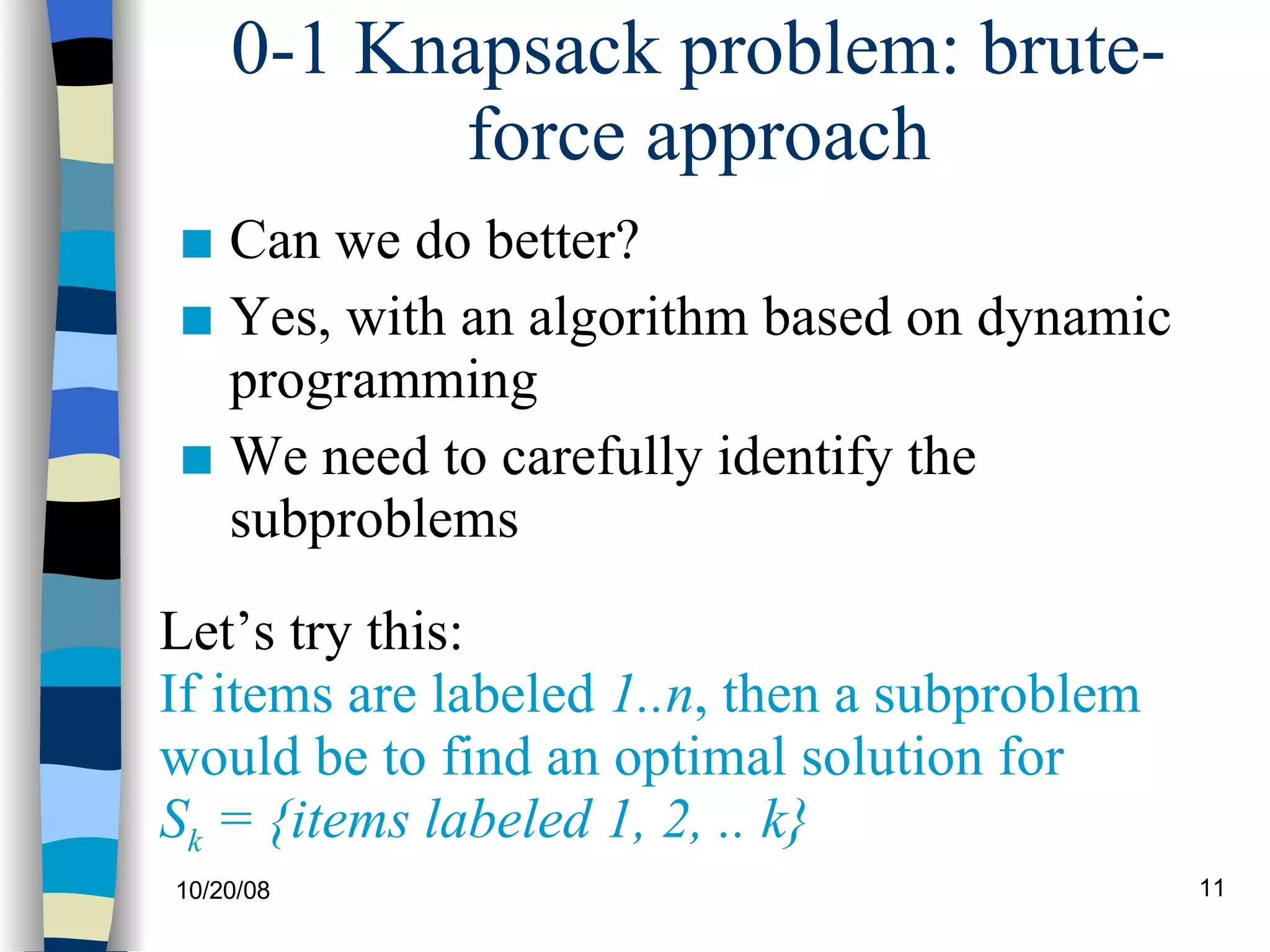
0-1 Knapsack problem: brute-force approach Can we do better?  Yes, with an algorithm based on dynamic programming We need to carefully identify the subproblems Let’s try this: If items are labeled  1..n , then a subproblem  would be to find an optimal solution for  S k  = {items labeled 1, 2, .. k}
Defining a Subproblem  If items are labeled  1..n , then a subproblem would be to find an optimal solution for  S k  = {items labeled 1, 2, .. k} This is a valid subproblem definition. The question is: can we describe the final solution ( S n   ) in terms of subproblems ( S k )?  Unfortunately, we  can’t  do that. Explanation follows….
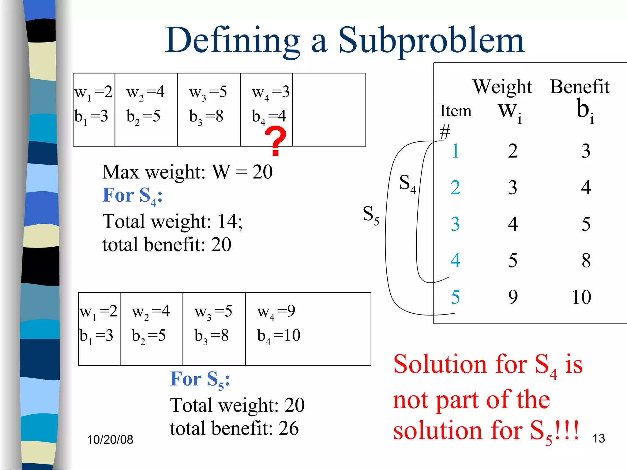
Defining a Subproblem Max weight: W = 20 For S 4 : Total weight: 14; total benefit: 20 w i b i 10 8 5 5 4 4 3 3 2 Weight Benefit 9 Item # 4 3 2 1 5 S 4 S 5 For S 5 : Total weight: 20 total benefit: 26 Solution for S 4  is not part of the solution for S 5 !!! ? w 1  =2 b 1  =3 w 2  =4 b 2  =5 w 3  =5 b 3  =8 w 4  =3 b 4  =4 w 1  =2 b 1  =3 w 2  =4 b 2  =5 w 3  =5 b 3  =8 w 4  =9 b 4  =10
Defining a Subproblem (continued) As we have seen, the solution for  S 4  is not part of the solution for  S 5 So our definition of a subproblem is flawed and we need another one! Let’s add another parameter:  w , which will represent the  exact  weight for each subset of items The subproblem then will be to compute  B[k,w]
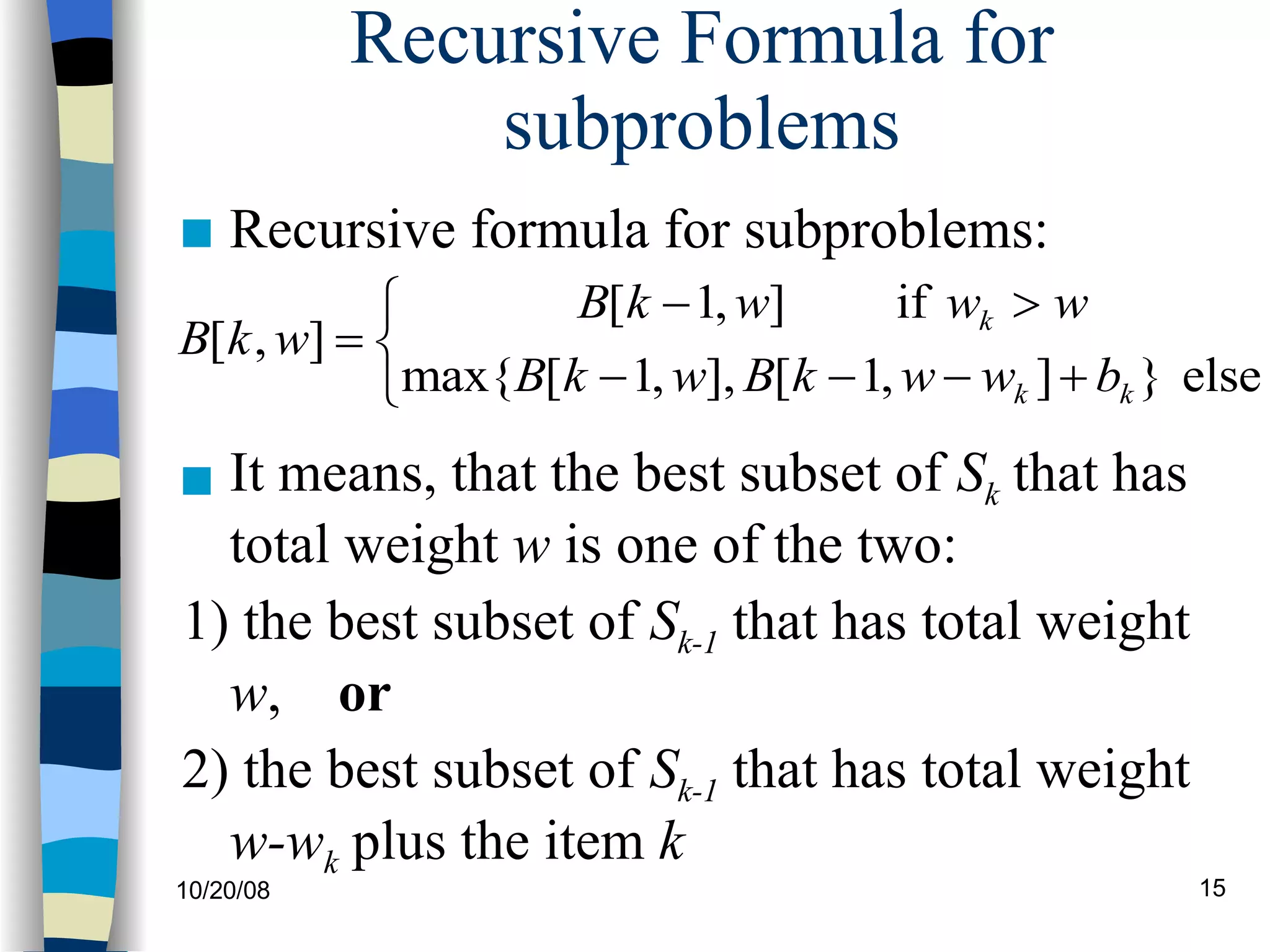
Recursive Formula for subproblems It means, that the best subset of  S k  that has total weight  w  is one of the two: 1) the best subset of  S k-1  that has total weight  w ,  or 2) the best subset of  S k-1  that has total weight  w-w k  plus the item  k Recursive formula for subproblems:
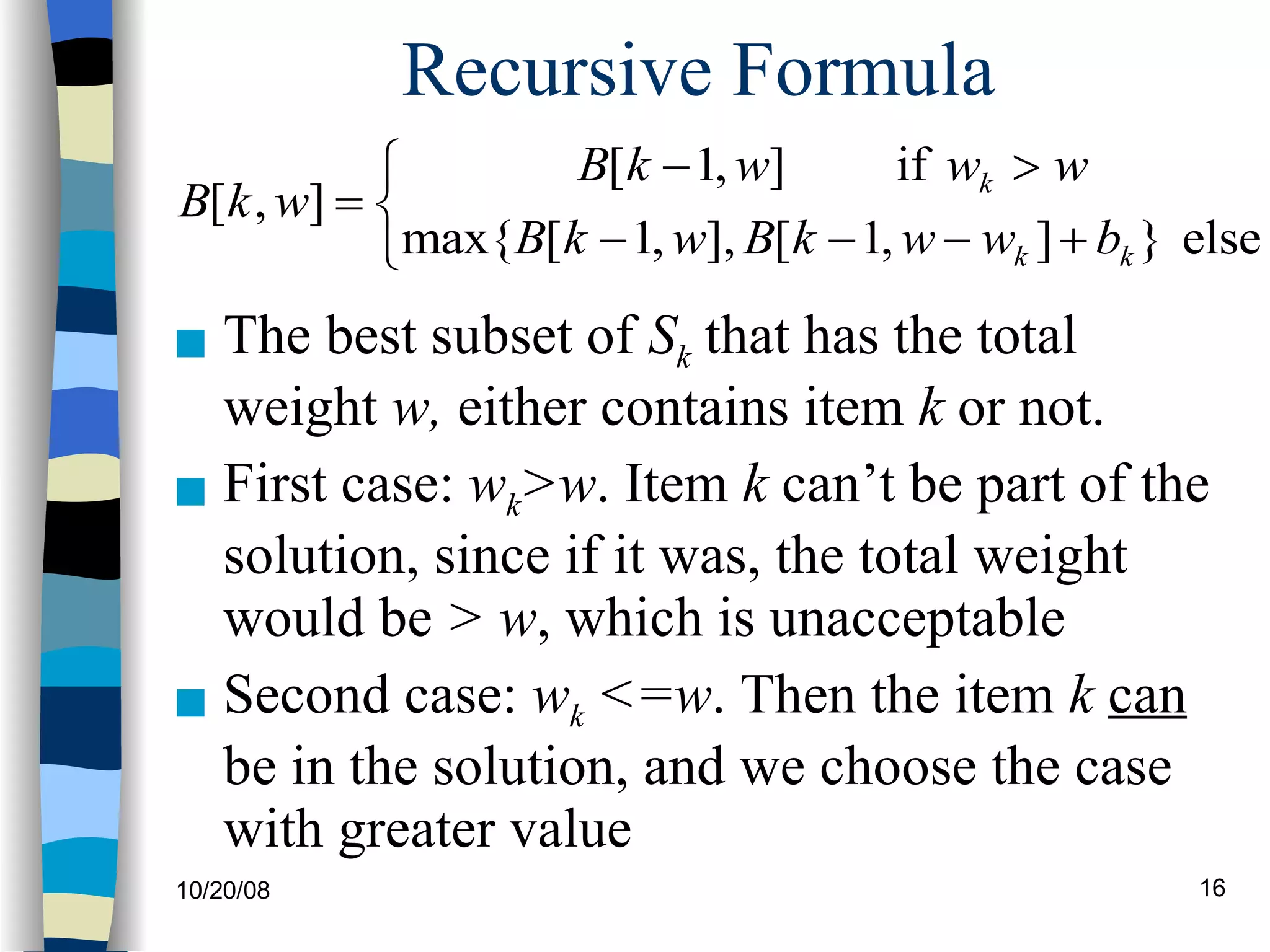
Recursive Formula The best subset of  S k  that has the total weight  w,  either contains item  k  or not. First case:  w k >w . Item  k  can’t be part of the solution, since if it was, the total weight would be  > w , which is unacceptable Second case:  w k  <=w . Then the item  k   can  be in the solution, and we choose the case with greater value
0-1 Knapsack Algorithm for w = 0 to W B[0,w] = 0 for i = 0 to n B[i,0] = 0 for w = 0 to W if w i  <= w  // item i can be part of the solution if b i  + B[i-1,w-w i ] > B[i-1,w] B[i,w] = b i  + B[i-1,w- w i ] else B[i,w] = B[i-1,w] else B[i,w] = B[i-1,w]  // w i  > w
Running time for w = 0 to W B[0,w] = 0 for i = 0 to n B[i,0] = 0 for w = 0 to W < the rest of the code > What is the running time of this algorithm? O(W) O(W) Repeat  n  times O(n*W) Remember that the brute-force algorithm  takes O(2 n )
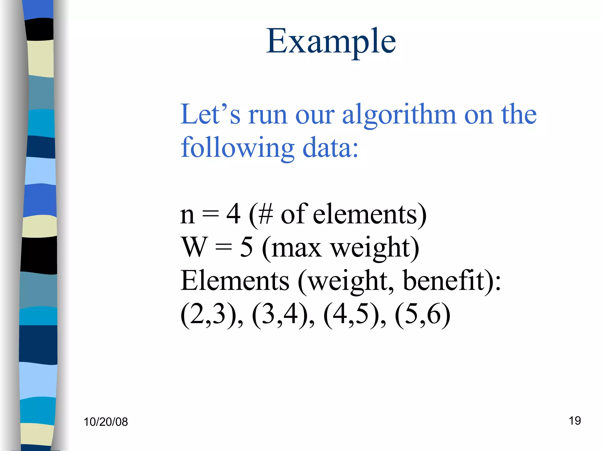
Example Let’s run our algorithm on the  following data: n = 4 (# of elements) W = 5 (max weight) Elements (weight, benefit): (2,3), (3,4), (4,5), (5,6)
Example (2) for w = 0 to W B[0,w] = 0 0 0 0 0 0 0 W 0 1 2 3 4 5 i 0 1 2 3 4
Example (3) for i = 0 to n B[i,0] = 0 0 0 0 0 0 0 W 0 1 2 3 4 5 i 0 1 2 3 0 0 0 0 4
Example (4) if w i  <= w  // item i can be part of the solution if b i  + B[i-1,w-w i ] > B[i-1,w] B[i,w] = b i  + B[i-1,w- w i ] else B[i,w] = B[i-1,w] else  B[i,w] = B[i-1,w]   // w i  > w  0 0 0 0 0 0 W 0 1 2 3 4 5 i 0 1 2 3 0 0 0 0 i=1 b i =3 w i =2 w= 1 w-w i  =-1 Items: 1: (2,3) 2: (3,4) 3: (4,5)  4: (5,6) 4 0
Example (5) if  w i  <= w   // item i can be part of the solution if  b i  + B[i-1,w-w i ] > B[i-1,w] B[i,w] = b i  + B[i-1,w- w i ] else B[i,w] = B[i-1,w] else B[i,w] = B[i-1,w]  // w i  > w  0 0 0 0 0 0 W 0 1 2 3 4 5 i 0 1 2 3 0 0 0 0 i=1 b i =3 w i =2 w= 2 w-w i  =0 Items: 1: (2,3) 2: (3,4) 3: (4,5)  4: (5,6) 4 0 3
Example (6) if  w i  <= w   // item i can be part of the solution if  b i  + B[i-1,w-w i ] > B[i-1,w] B[i,w] = b i  + B[i-1,w- w i ] else B[i,w] = B[i-1,w] else B[i,w] = B[i-1,w]  // w i  > w  0 0 0 0 0 0 W 0 1 2 3 4 5 i 0 1 2 3 0 0 0 0 i=1 b i =3 w i =2 w= 3 w-w i =1 Items: 1: (2,3) 2: (3,4) 3: (4,5)  4: (5,6) 4 0 3 3
Example (7) if  w i  <= w   // item i can be part of the solution if  b i  + B[i-1,w-w i ] > B[i-1,w] B[i,w] = b i  + B[i-1,w- w i ] else B[i,w] = B[i-1,w] else B[i,w] = B[i-1,w]  // w i  > w  0 0 0 0 0 0 W 0 1 2 3 4 5 i 0 1 2 3 0 0 0 0 i=1 b i =3 w i =2 w= 4 w-w i =2 Items: 1: (2,3) 2: (3,4) 3: (4,5)  4: (5,6) 4 0 3 3 3
Example (8) if  w i  <= w   // item i can be part of the solution if  b i  + B[i-1,w-w i ] > B[i-1,w] B[i,w] = b i  + B[i-1,w- w i ] else B[i,w] = B[i-1,w] else B[i,w] = B[i-1,w]  // w i  > w  0 0 0 0 0 0 W 0 1 2 3 4 5 i 0 1 2 3 0 0 0 0 i=1 b i =3 w i =2 w= 5 w-w i =2 Items: 1: (2,3) 2: (3,4) 3: (4,5)  4: (5,6) 4 0 3 3 3 3
Example (9) if w i  <= w  // item i can be part of the solution if b i  + B[i-1,w-w i ] > B[i-1,w] B[i,w] = b i  + B[i-1,w- w i ] else B[i,w] = B[i-1,w] else   B[i,w] = B[i-1,w]   // w i  > w  0 0 0 0 0 0 W 0 1 2 3 4 5 i 0 1 2 3 0 0 0 0 i=2 b i =4 w i =3 w= 1 w-w i =-2 Items: 1: (2,3) 2: (3,4) 3: (4,5)  4: (5,6) 4 0 3 3 3 3 0
Example (10) if w i  <= w  // item i can be part of the solution if b i  + B[i-1,w-w i ] > B[i-1,w] B[i,w] = b i  + B[i-1,w- w i ] else B[i,w] = B[i-1,w] else   B[i,w] = B[i-1,w]   // w i  > w  0 0 0 0 0 0 W 0 1 2 3 4 5 i 0 1 2 3 0 0 0 0 i=2 b i =4 w i =3 w= 2 w-w i =-1 Items: 1: (2,3) 2: (3,4) 3: (4,5)  4: (5,6) 4 0 3 3 3 3 0 3
Example (11) if  w i  <= w   // item i can be part of the solution if  b i  + B[i-1,w-w i ] > B[i-1,w] B[i,w] = b i  + B[i-1,w- w i ] else B[i,w] = B[i-1,w] else B[i,w] = B[i-1,w]  // w i  > w  0 0 0 0 0 0 W 0 1 2 3 4 5 i 0 1 2 3 0 0 0 0 i=2 b i =4 w i =3 w= 3 w-w i =0 Items: 1: (2,3) 2: (3,4) 3: (4,5)  4: (5,6) 4 0 3 3 3 3 0 3 4
Example (12) if  w i  <= w   // item i can be part of the solution if  b i  + B[i-1,w-w i ] > B[i-1,w] B[i,w] = b i  + B[i-1,w- w i ] else B[i,w] = B[i-1,w] else B[i,w] = B[i-1,w]  // w i  > w  0 0 0 0 0 0 W 0 1 2 3 4 5 i 0 1 2 3 0 0 0 0 i=2 b i =4 w i =3 w= 4 w-w i =1 Items: 1: (2,3) 2: (3,4) 3: (4,5)  4: (5,6) 4 0 3 3 3 3 0 3 4 4
Example (13) if  w i  <= w   // item i can be part of the solution if  b i  + B[i-1,w-w i ] > B[i-1,w] B[i,w] = b i  + B[i-1,w- w i ] else B[i,w] = B[i-1,w] else B[i,w] = B[i-1,w]  // w i  > w  0 0 0 0 0 0 W 0 1 2 3 4 5 i 0 1 2 3 0 0 0 0 i=2 b i =4 w i =3 w= 5 w-w i =2 Items: 1: (2,3) 2: (3,4) 3: (4,5)  4: (5,6) 4 0 3 3 3 3 0 3 4 4 7
Example (14) if w i  <= w  // item i can be part of the solution if b i  + B[i-1,w-w i ] > B[i-1,w] B[i,w] = b i  + B[i-1,w- w i ] else B[i,w] = B[i-1,w] else   B[i,w] = B[i-1,w]   // w i  > w  0 0 0 0 0 0 W 0 1 2 3 4 5 i 0 1 2 3 0 0 0 0 i=3 b i =5 w i =4 w= 1..3 Items: 1: (2,3) 2: (3,4) 3: (4,5)  4: (5,6) 4 0 3 3 3 3 0 0 3 4 4 7 0 3 4
Example (15) if  w i  <= w   // item i can be part of the solution if  b i  + B[i-1,w-w i ] > B[i-1,w] B[i,w] = b i  + B[i-1,w- w i ] else B[i,w] = B[i-1,w] else B[i,w] = B[i-1,w]  // w i  > w  0 0 0 0 0 0 W 0 1 2 3 4 5 i 0 1 2 3 0 0 0 0 i=3 b i =5 w i =4 w= 4 w- w i =0 Items: 1: (2,3) 2: (3,4) 3: (4,5)  4: (5,6) 4 0 0 0 3 4 4 7 0 3 4 5 3 3 3 3
Example (15) if  w i  <= w   // item i can be part of the solution if b i  + B[i-1,w-w i ] > B[i-1,w] B[i,w] = b i  + B[i-1,w- w i ] else B[i,w] = B[i-1,w] else B[i,w] = B[i-1,w]  // w i  > w  0 0 0 0 0 0 W 0 1 2 3 4 5 i 0 1 2 3 0 0 0 0 i=3 b i =5 w i =4 w= 5 w- w i =1 Items: 1: (2,3) 2: (3,4) 3: (4,5)  4: (5,6) 4 0 0 0 3 4 4 7 0 3 4 5 7 3 3 3 3
Example (16) if w i  <= w  // item i can be part of the solution if b i  + B[i-1,w-w i ] > B[i-1,w] B[i,w] = b i  + B[i-1,w- w i ] else B[i,w] = B[i-1,w] else  B[i,w] = B[i-1,w]   // w i  > w  0 0 0 0 0 0 W 0 1 2 3 4 5 i 0 1 2 3 0 0 0 0 i=3 b i =5 w i =4 w= 1..4 Items: 1: (2,3) 2: (3,4) 3: (4,5)  4: (5,6) 4 0 0 0 3 4 4 7 0 3 4 5 7 0 3 4 5 3 3 3 3
Example (17) if  w i  <= w   // item i can be part of the solution if b i  + B[i-1,w-w i ] > B[i-1,w] B[i,w] = b i  + B[i-1,w- w i ] else B[i,w] = B[i-1,w] else B[i,w] = B[i-1,w]  // w i  > w  0 0 0 0 0 0 W 0 1 2 3 4 5 i 0 1 2 3 0 0 0 0 i=3 b i =5 w i =4 w= 5 Items: 1: (2,3) 2: (3,4) 3: (4,5)  4: (5,6) 4 0 0 0 3 4 4 7 0 3 4 5 7 0 3 4 5 7 3 3 3 3
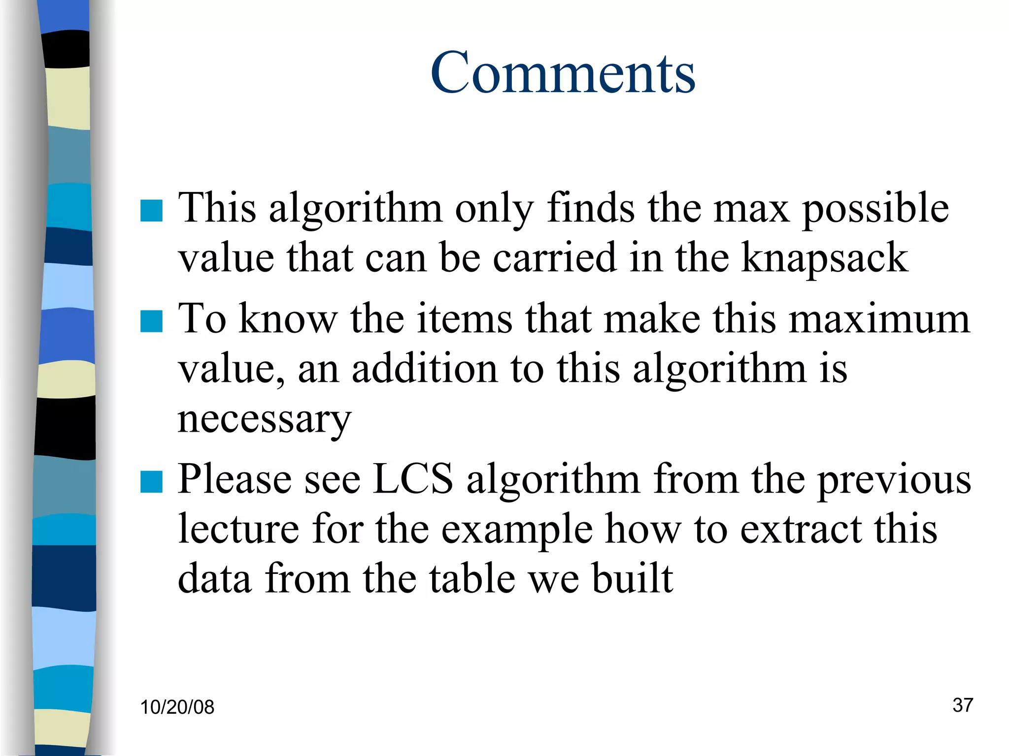
Comments This algorithm only finds the max possible value that can be carried in the knapsack To know the items that make this maximum value, an addition to this algorithm is necessary Please see LCS algorithm from the previous lecture for the example how to extract this data from the table we built
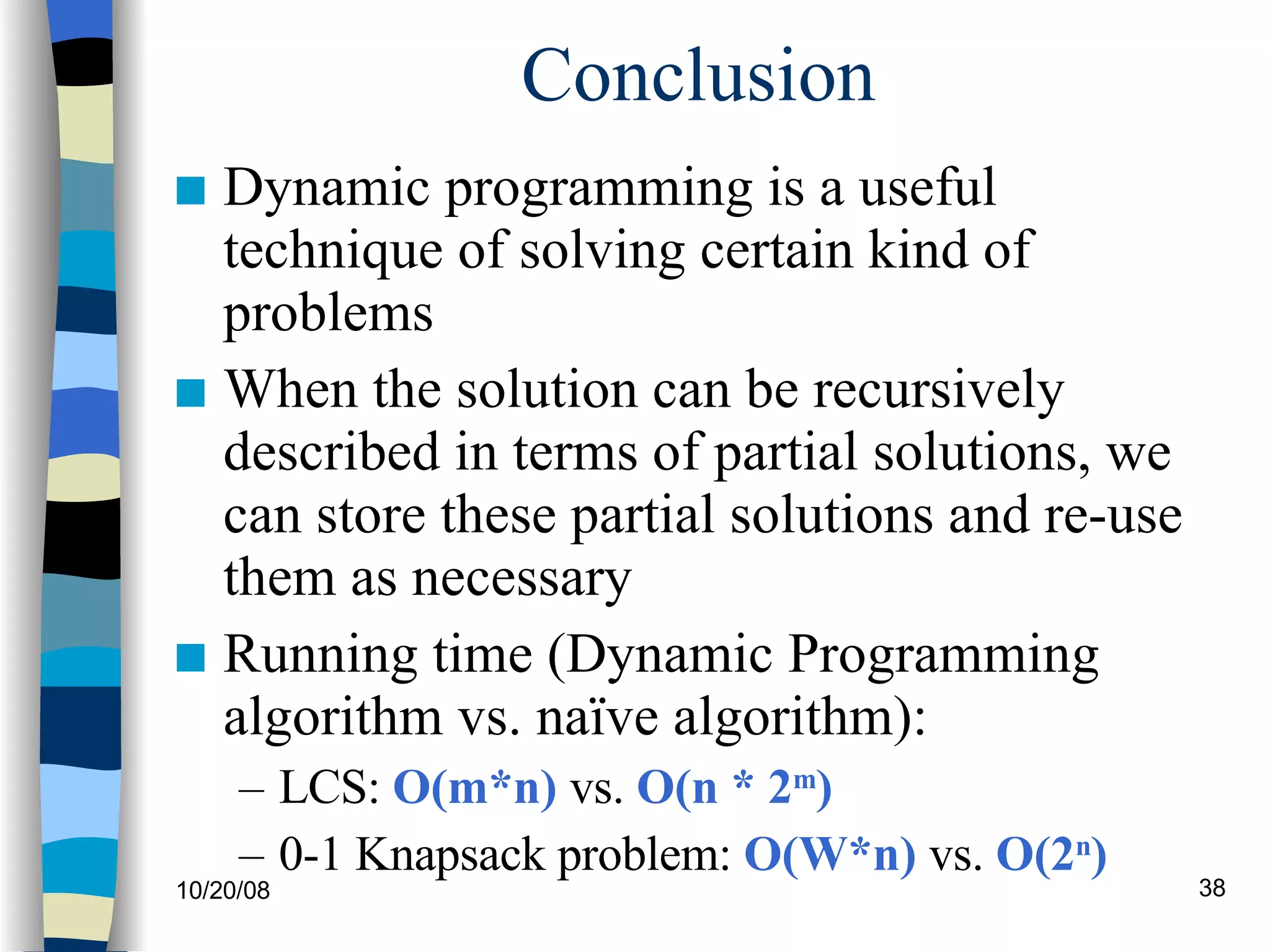
Conclusion Dynamic programming is a useful technique of solving certain kind of problems When the solution can be recursively described in terms of partial solutions, we can store these partial solutions and re-use them as necessary Running time (Dynamic Programming algorithm vs. naïve algorithm): LCS:  O(m*n)  vs.  O(n * 2 m ) 0-1 Knapsack problem:  O(W*n)  vs.  O(2 n )
The End

lecture 25

  • 1.
    CS 332 -Algorithms Dynamic programming 0-1 Knapsack problem
  • 2.
    Review: Dynamic programmingDP is a method for solving certain kind of problems DP can be applied when the solution of a problem includes solutions to subproblems We need to find a recursive formula for the solution We can recursively solve subproblems, starting from the trivial case, and save their solutions in memory In the end we’ll get the solution of the whole problem
  • 3.
    Properties of aproblem that can be solved with dynamic programming Simple Subproblems We should be able to break the original problem to smaller subproblems that have the same structure Optimal Substructure of the problems The solution to the problem must be a composition of subproblem solutions Subproblem Overlap Optimal subproblems to unrelated problems can contain subproblems in common
  • 4.
    Review: LongestCommon Subsequence (LCS) Problem: how to find the longest pattern of characters that is common to two text strings X and Y Dynamic programming algorithm: solve subproblems until we get the final solution Subproblem: first find the LCS of prefixes of X and Y. this problem has optimal substructure : LCS of two prefixes is always a part of LCS of bigger strings
  • 5.
    Review: LongestCommon Subsequence (LCS) continued Define X i , Y j to be prefixes of X and Y of length i and j; m = |X|, n = |Y| We store the length of LCS(X i , Y j ) in c[i,j] Trivial cases: LCS(X 0 , Y j ) and LCS(X i , Y 0 ) is empty (so c[0,j] = c[i,0] = 0 ) Recursive formula for c[i,j]: c[m,n] is the final solution
  • 6.
    Review: LongestCommon Subsequence (LCS) After we have filled the array c[ ], we can use this data to find the characters that constitute the Longest Common Subsequence Algorithm runs in O(m*n) , which is much better than the brute-force algorithm: O(n 2 m )
  • 7.
    0-1 Knapsack problemGiven a knapsack with maximum capacity W , and a set S consisting of n items Each item i has some weight w i and benefit value b i (all w i , b i and W are integer values) Problem : How to pack the knapsack to achieve maximum total value of packed items?
  • 8.
    0-1 Knapsack problem:a picture w i b i 10 9 8 5 5 4 4 3 3 2 Weight Benefit value This is a knapsack Max weight: W = 20 Items W = 20
  • 9.
    0-1 Knapsack problemProblem, in other words, is to find The problem is called a “0-1” problem, because each item must be entirely accepted or rejected. Just another version of this problem is the “ Fractional Knapsack Problem ”, where we can take fractions of items.
  • 10.
    0-1 Knapsack problem:brute-force approach Let’s first solve this problem with a straightforward algorithm Since there are n items, there are 2 n possible combinations of items. We go through all combinations and find the one with the most total value and with total weight less or equal to W Running time will be O(2 n )
  • 11.
    0-1 Knapsack problem:brute-force approach Can we do better? Yes, with an algorithm based on dynamic programming We need to carefully identify the subproblems Let’s try this: If items are labeled 1..n , then a subproblem would be to find an optimal solution for S k = {items labeled 1, 2, .. k}
  • 12.
    Defining a Subproblem If items are labeled 1..n , then a subproblem would be to find an optimal solution for S k = {items labeled 1, 2, .. k} This is a valid subproblem definition. The question is: can we describe the final solution ( S n ) in terms of subproblems ( S k )? Unfortunately, we can’t do that. Explanation follows….
  • 13.
    Defining a SubproblemMax weight: W = 20 For S 4 : Total weight: 14; total benefit: 20 w i b i 10 8 5 5 4 4 3 3 2 Weight Benefit 9 Item # 4 3 2 1 5 S 4 S 5 For S 5 : Total weight: 20 total benefit: 26 Solution for S 4 is not part of the solution for S 5 !!! ? w 1 =2 b 1 =3 w 2 =4 b 2 =5 w 3 =5 b 3 =8 w 4 =3 b 4 =4 w 1 =2 b 1 =3 w 2 =4 b 2 =5 w 3 =5 b 3 =8 w 4 =9 b 4 =10
  • 14.
    Defining a Subproblem(continued) As we have seen, the solution for S 4 is not part of the solution for S 5 So our definition of a subproblem is flawed and we need another one! Let’s add another parameter: w , which will represent the exact weight for each subset of items The subproblem then will be to compute B[k,w]
  • 15.
    Recursive Formula forsubproblems It means, that the best subset of S k that has total weight w is one of the two: 1) the best subset of S k-1 that has total weight w , or 2) the best subset of S k-1 that has total weight w-w k plus the item k Recursive formula for subproblems:
  • 16.
    Recursive Formula Thebest subset of S k that has the total weight w, either contains item k or not. First case: w k >w . Item k can’t be part of the solution, since if it was, the total weight would be > w , which is unacceptable Second case: w k <=w . Then the item k can be in the solution, and we choose the case with greater value
  • 17.
    0-1 Knapsack Algorithmfor w = 0 to W B[0,w] = 0 for i = 0 to n B[i,0] = 0 for w = 0 to W if w i <= w // item i can be part of the solution if b i + B[i-1,w-w i ] > B[i-1,w] B[i,w] = b i + B[i-1,w- w i ] else B[i,w] = B[i-1,w] else B[i,w] = B[i-1,w] // w i > w
  • 18.
    Running time forw = 0 to W B[0,w] = 0 for i = 0 to n B[i,0] = 0 for w = 0 to W < the rest of the code > What is the running time of this algorithm? O(W) O(W) Repeat n times O(n*W) Remember that the brute-force algorithm takes O(2 n )
  • 19.
    Example Let’s runour algorithm on the following data: n = 4 (# of elements) W = 5 (max weight) Elements (weight, benefit): (2,3), (3,4), (4,5), (5,6)
  • 20.
    Example (2) forw = 0 to W B[0,w] = 0 0 0 0 0 0 0 W 0 1 2 3 4 5 i 0 1 2 3 4
  • 21.
    Example (3) fori = 0 to n B[i,0] = 0 0 0 0 0 0 0 W 0 1 2 3 4 5 i 0 1 2 3 0 0 0 0 4
  • 22.
    Example (4) ifw i <= w // item i can be part of the solution if b i + B[i-1,w-w i ] > B[i-1,w] B[i,w] = b i + B[i-1,w- w i ] else B[i,w] = B[i-1,w] else B[i,w] = B[i-1,w] // w i > w 0 0 0 0 0 0 W 0 1 2 3 4 5 i 0 1 2 3 0 0 0 0 i=1 b i =3 w i =2 w= 1 w-w i =-1 Items: 1: (2,3) 2: (3,4) 3: (4,5) 4: (5,6) 4 0
  • 23.
    Example (5) if w i <= w // item i can be part of the solution if b i + B[i-1,w-w i ] > B[i-1,w] B[i,w] = b i + B[i-1,w- w i ] else B[i,w] = B[i-1,w] else B[i,w] = B[i-1,w] // w i > w 0 0 0 0 0 0 W 0 1 2 3 4 5 i 0 1 2 3 0 0 0 0 i=1 b i =3 w i =2 w= 2 w-w i =0 Items: 1: (2,3) 2: (3,4) 3: (4,5) 4: (5,6) 4 0 3
  • 24.
    Example (6) if w i <= w // item i can be part of the solution if b i + B[i-1,w-w i ] > B[i-1,w] B[i,w] = b i + B[i-1,w- w i ] else B[i,w] = B[i-1,w] else B[i,w] = B[i-1,w] // w i > w 0 0 0 0 0 0 W 0 1 2 3 4 5 i 0 1 2 3 0 0 0 0 i=1 b i =3 w i =2 w= 3 w-w i =1 Items: 1: (2,3) 2: (3,4) 3: (4,5) 4: (5,6) 4 0 3 3
  • 25.
    Example (7) if w i <= w // item i can be part of the solution if b i + B[i-1,w-w i ] > B[i-1,w] B[i,w] = b i + B[i-1,w- w i ] else B[i,w] = B[i-1,w] else B[i,w] = B[i-1,w] // w i > w 0 0 0 0 0 0 W 0 1 2 3 4 5 i 0 1 2 3 0 0 0 0 i=1 b i =3 w i =2 w= 4 w-w i =2 Items: 1: (2,3) 2: (3,4) 3: (4,5) 4: (5,6) 4 0 3 3 3
  • 26.
    Example (8) if w i <= w // item i can be part of the solution if b i + B[i-1,w-w i ] > B[i-1,w] B[i,w] = b i + B[i-1,w- w i ] else B[i,w] = B[i-1,w] else B[i,w] = B[i-1,w] // w i > w 0 0 0 0 0 0 W 0 1 2 3 4 5 i 0 1 2 3 0 0 0 0 i=1 b i =3 w i =2 w= 5 w-w i =2 Items: 1: (2,3) 2: (3,4) 3: (4,5) 4: (5,6) 4 0 3 3 3 3
  • 27.
    Example (9) ifw i <= w // item i can be part of the solution if b i + B[i-1,w-w i ] > B[i-1,w] B[i,w] = b i + B[i-1,w- w i ] else B[i,w] = B[i-1,w] else B[i,w] = B[i-1,w] // w i > w 0 0 0 0 0 0 W 0 1 2 3 4 5 i 0 1 2 3 0 0 0 0 i=2 b i =4 w i =3 w= 1 w-w i =-2 Items: 1: (2,3) 2: (3,4) 3: (4,5) 4: (5,6) 4 0 3 3 3 3 0
  • 28.
    Example (10) ifw i <= w // item i can be part of the solution if b i + B[i-1,w-w i ] > B[i-1,w] B[i,w] = b i + B[i-1,w- w i ] else B[i,w] = B[i-1,w] else B[i,w] = B[i-1,w] // w i > w 0 0 0 0 0 0 W 0 1 2 3 4 5 i 0 1 2 3 0 0 0 0 i=2 b i =4 w i =3 w= 2 w-w i =-1 Items: 1: (2,3) 2: (3,4) 3: (4,5) 4: (5,6) 4 0 3 3 3 3 0 3
  • 29.
    Example (11) if w i <= w // item i can be part of the solution if b i + B[i-1,w-w i ] > B[i-1,w] B[i,w] = b i + B[i-1,w- w i ] else B[i,w] = B[i-1,w] else B[i,w] = B[i-1,w] // w i > w 0 0 0 0 0 0 W 0 1 2 3 4 5 i 0 1 2 3 0 0 0 0 i=2 b i =4 w i =3 w= 3 w-w i =0 Items: 1: (2,3) 2: (3,4) 3: (4,5) 4: (5,6) 4 0 3 3 3 3 0 3 4
  • 30.
    Example (12) if w i <= w // item i can be part of the solution if b i + B[i-1,w-w i ] > B[i-1,w] B[i,w] = b i + B[i-1,w- w i ] else B[i,w] = B[i-1,w] else B[i,w] = B[i-1,w] // w i > w 0 0 0 0 0 0 W 0 1 2 3 4 5 i 0 1 2 3 0 0 0 0 i=2 b i =4 w i =3 w= 4 w-w i =1 Items: 1: (2,3) 2: (3,4) 3: (4,5) 4: (5,6) 4 0 3 3 3 3 0 3 4 4
  • 31.
    Example (13) if w i <= w // item i can be part of the solution if b i + B[i-1,w-w i ] > B[i-1,w] B[i,w] = b i + B[i-1,w- w i ] else B[i,w] = B[i-1,w] else B[i,w] = B[i-1,w] // w i > w 0 0 0 0 0 0 W 0 1 2 3 4 5 i 0 1 2 3 0 0 0 0 i=2 b i =4 w i =3 w= 5 w-w i =2 Items: 1: (2,3) 2: (3,4) 3: (4,5) 4: (5,6) 4 0 3 3 3 3 0 3 4 4 7
  • 32.
    Example (14) ifw i <= w // item i can be part of the solution if b i + B[i-1,w-w i ] > B[i-1,w] B[i,w] = b i + B[i-1,w- w i ] else B[i,w] = B[i-1,w] else B[i,w] = B[i-1,w] // w i > w 0 0 0 0 0 0 W 0 1 2 3 4 5 i 0 1 2 3 0 0 0 0 i=3 b i =5 w i =4 w= 1..3 Items: 1: (2,3) 2: (3,4) 3: (4,5) 4: (5,6) 4 0 3 3 3 3 0 0 3 4 4 7 0 3 4
  • 33.
    Example (15) if w i <= w // item i can be part of the solution if b i + B[i-1,w-w i ] > B[i-1,w] B[i,w] = b i + B[i-1,w- w i ] else B[i,w] = B[i-1,w] else B[i,w] = B[i-1,w] // w i > w 0 0 0 0 0 0 W 0 1 2 3 4 5 i 0 1 2 3 0 0 0 0 i=3 b i =5 w i =4 w= 4 w- w i =0 Items: 1: (2,3) 2: (3,4) 3: (4,5) 4: (5,6) 4 0 0 0 3 4 4 7 0 3 4 5 3 3 3 3
  • 34.
    Example (15) if w i <= w // item i can be part of the solution if b i + B[i-1,w-w i ] > B[i-1,w] B[i,w] = b i + B[i-1,w- w i ] else B[i,w] = B[i-1,w] else B[i,w] = B[i-1,w] // w i > w 0 0 0 0 0 0 W 0 1 2 3 4 5 i 0 1 2 3 0 0 0 0 i=3 b i =5 w i =4 w= 5 w- w i =1 Items: 1: (2,3) 2: (3,4) 3: (4,5) 4: (5,6) 4 0 0 0 3 4 4 7 0 3 4 5 7 3 3 3 3
  • 35.
    Example (16) ifw i <= w // item i can be part of the solution if b i + B[i-1,w-w i ] > B[i-1,w] B[i,w] = b i + B[i-1,w- w i ] else B[i,w] = B[i-1,w] else B[i,w] = B[i-1,w] // w i > w 0 0 0 0 0 0 W 0 1 2 3 4 5 i 0 1 2 3 0 0 0 0 i=3 b i =5 w i =4 w= 1..4 Items: 1: (2,3) 2: (3,4) 3: (4,5) 4: (5,6) 4 0 0 0 3 4 4 7 0 3 4 5 7 0 3 4 5 3 3 3 3
  • 36.
    Example (17) if w i <= w // item i can be part of the solution if b i + B[i-1,w-w i ] > B[i-1,w] B[i,w] = b i + B[i-1,w- w i ] else B[i,w] = B[i-1,w] else B[i,w] = B[i-1,w] // w i > w 0 0 0 0 0 0 W 0 1 2 3 4 5 i 0 1 2 3 0 0 0 0 i=3 b i =5 w i =4 w= 5 Items: 1: (2,3) 2: (3,4) 3: (4,5) 4: (5,6) 4 0 0 0 3 4 4 7 0 3 4 5 7 0 3 4 5 7 3 3 3 3
  • 37.
    Comments This algorithmonly finds the max possible value that can be carried in the knapsack To know the items that make this maximum value, an addition to this algorithm is necessary Please see LCS algorithm from the previous lecture for the example how to extract this data from the table we built
  • 38.
    Conclusion Dynamic programmingis a useful technique of solving certain kind of problems When the solution can be recursively described in terms of partial solutions, we can store these partial solutions and re-use them as necessary Running time (Dynamic Programming algorithm vs. naïve algorithm): LCS: O(m*n) vs. O(n * 2 m ) 0-1 Knapsack problem: O(W*n) vs. O(2 n )
  • 39.