Introduction to R
Andrew Zieffler
Some Things to Remember...
• R is case-sensitive
anova is different than Anova is different than ANOVA
• R does exactly what the user codes
• R has a "long-term" memory...
The user and R often don’t see “eye-to-eye”
...but only in the current session
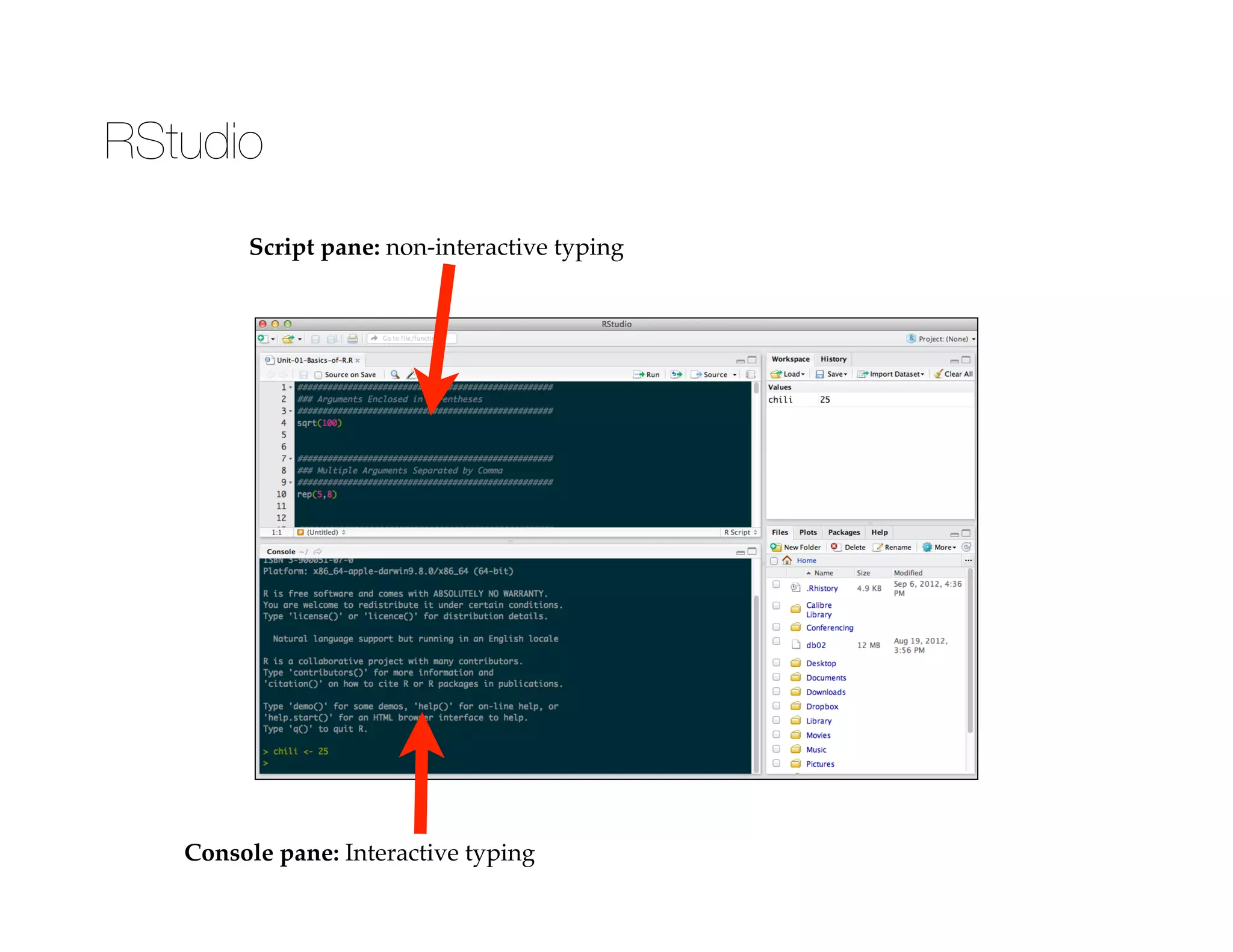
RStudio
Console pane: Interactive typing
Script pane: non-interactive typing
>
Console Pane (Interactive)
R prompt...R is waiting for a command
> 3 + 2
!
[1] 5
After inputting a command hit <enter>
R returned value...the brackets indicate the ith returned element.!
Here they indicate the first returned element.!
(They can be ignored for now (we are more interested in the returned value of 5.)
> 3 +
!
+
Continuation prompt... The previous command was not
properly ended prior to hitting <enter>!
!
• Finish command!
• Hit <esc> until you get the command prompt again.
Then re-try
{Two options
> 4 * 5
[1] 20
!
> 10 ^ 3
[1] 1000
!
> 1 / 0
[1] Inf
Space is for humans.
> 4 * 5
> 4*5
> 4 *5
are all the same to R
> sqrt(100)
[1] 10
!
> log(7)
[1] 1.94591
!
> sin(50)
[1] -0.2623749
!
> exp(3)
[1] 20.08554
!
> log(100, 10)
[1] 2
!
> log(100, base = 10)
[1] 2
Three components!
• Function!
• Argument!
• Returned value
Arguments!
Enclosed in parentheses
Multiple arguments
separated by commas
Can be named or unnamed
Computations in R using Functions
> log(100, 10)
[1] 2
!
> log(10, 100)
[1] 0.5
!
> log(x = 100, base = 10)
[1] 2
!
> log(base = 10, x = 100)
[1] 2
!
> log(100, base = 10)
[1] 2
Order does not matter for
named arguments
Conventionally, the first
argument is often unnamed
and the remainder are named
Order matters for unnamed
arguments
Connecting Computations in R
Two methods of connecting computations !
• Chaining!
• Assignment
!
> sqrt( log(100, base = 10) )
!
[1] 1.414214
!
> chili <- log(100, base = 10)
> chili = log(100, base = 10)
!
> sqrt(chili)
[1] 1.414214
Chaining uses a complete computation as the
argument for another computation.
Assignment stores the returned value from a
computation as a named object.
The assignment operator is
either <- or =
> chili = 3
!
> sqrt(chili)
[1] 1.732051
!
> chili
[1] 3
When an object name is re-used, the
previous value of the object is lost.
Workspace: List of current objects
• Pretty much any name can be used!
• Descriptive is better!
‣ chili is not a good object name!
• Names cannot include hyphens or
spaces!
• Names cannot begin with a digit!
• Conventions in CS!
‣ myData (bumpy/camel-case)!
‣ my_data (use underscore/period)
Objects
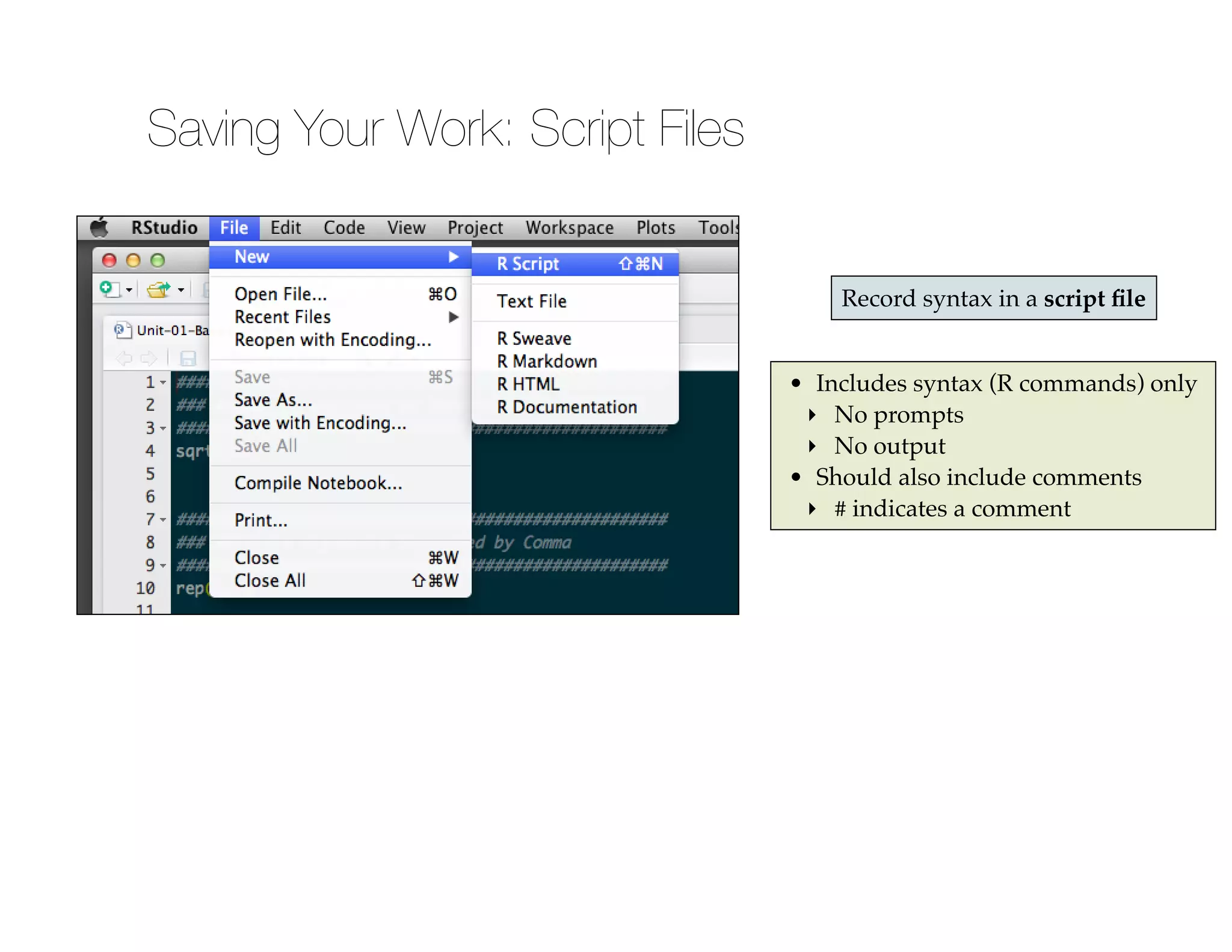
Saving Your Work: Script Files
Record syntax in a script file
• Includes syntax (R commands) only!
‣ No prompts!
‣ No output!
• Should also include comments!
‣ # indicates a comment
# Arithmetic computations
3 + 2
4 * 5
10 ^ 3
!
# Assignment
chili = log(100, base = 10)
!
# Compute things
sqrt(chili) # Find the square root
log(chili) # Find the natural logarithm
good script files have
comments
Comments can also be
placed on an existing line
Syntax in the script file can be
executed by highlighting it and
pressing the Run button!
!
Vectors are collections of data (univariate; a single
variable). They are typically assigned to an object. To
create a vector use the c() function.
> age = c(40, 37, 9, 2, 10)
!
> age
[1] 40 37 9 2 10
!
> age + 5
[1] 45 42 14 7 15
!
> age ^ 2
[1] 1600 1369 81 4 100
!
> mean(age)
[1] 19.6
!
> sum(age)
[1] 98
Some computations are
element-wise
Some computations are
vector-wise
Data Structures: Vectors
Not all vectors are numeric. R has six
different types of vectors. Use class()
to find out what type you have.
> family = c("Andy", "Lauren", "Chili", "Sadie", "Einstein")
!
> family
[1] "Andy" "Lauren" "Chili" "Sadie" "Einstein"
!
> family + 5
Error in family + 5 : non-numeric argument to binary operator
!
> length(family)
[1] 5
!
> family2 = c("Andy", "Lauren", "Chili", 1, 5)
!
> family2
[1] "Andy" "Lauren" "Chili" "1" "5"
In a character vector (a.k.a.
strings, literals) each element is a
character string. Character strings
are delimited by quotation marks.
All elements in a vector
have to be of the same
type...if not they will be
coerced to the same type
Character Vectors
> myLogical = c(TRUE, FALSE, FALSE)
!
> age
[1] 40 37 9 2 10
!
> age > 10
[1] TRUE TRUE FALSE FALSE FALSE
!
> people = (age > 10)
!
> length(people)
[1] 5
!
> people + 1
[1] 2 2 1 1 1
In a logical vector each element is TRUE
or FALSE. Logical elements are not
delimited by quotation marks.
Logical vectors are often
generated through
conditional statements
Logical elements have
numeric values associated
with them, namely 0
(FALSE) or 1 (TRUE).
Logical Vectors
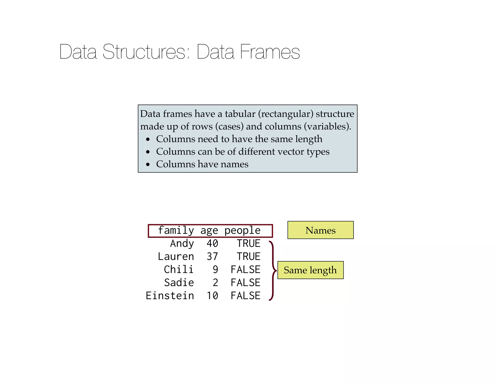
Data frames have a tabular (rectangular) structure
made up of rows (cases) and columns (variables).!
• Columns need to have the same length!
• Columns can be of different vector types!
• Columns have names
family age people
Andy 40 TRUE
Lauren 37 TRUE
Chili 9 FALSE
Sadie 2 FALSE
Einstein 10 FALSE
}Same length
Names
Data Structures: Data Frames
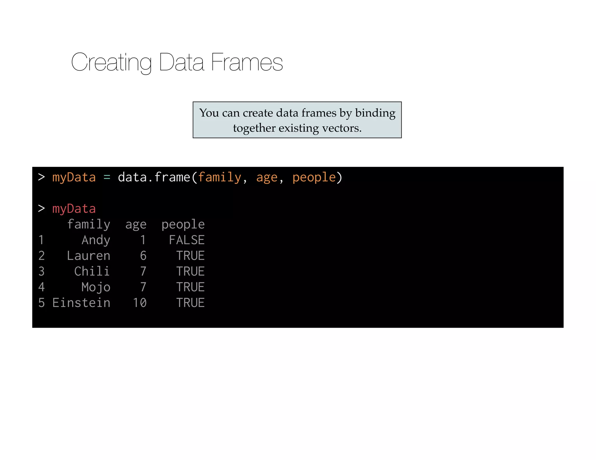
> myData = data.frame(family, age, people)
!
> myData
family age people
1 Andy 1 FALSE
2 Lauren 6 TRUE
3 Chili 7 TRUE
4 Mojo 7 TRUE
5 Einstein 10 TRUE
You can create data frames by binding
together existing vectors.
Creating Data Frames
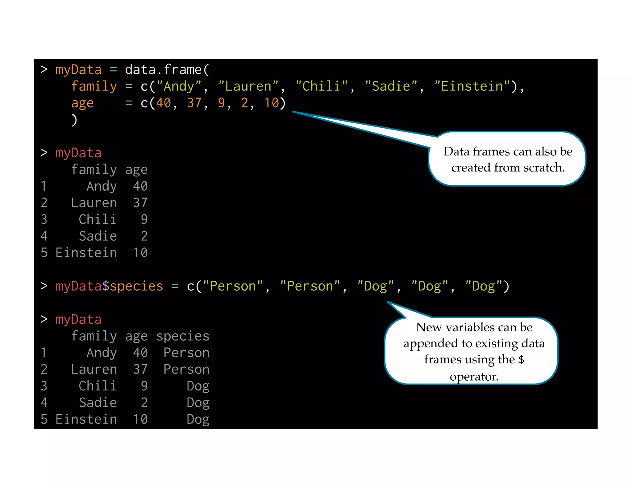
> myData = data.frame(
family = c("Andy", "Lauren", "Chili", "Sadie", "Einstein"),
age = c(40, 37, 9, 2, 10)
)
!
> myData
family age
1 Andy 40
2 Lauren 37
3 Chili 9
4 Sadie 2
5 Einstein 10
!
> myData$species = c("Person", "Person", "Dog", "Dog", "Dog")
!
> myData
family age species
1 Andy 40 Person
2 Lauren 37 Person
3 Chili 9 Dog
4 Sadie 2 Dog
5 Einstein 10 Dog
Data frames can also be
created from scratch.
New variables can be
appended to existing data
frames using the $
operator.
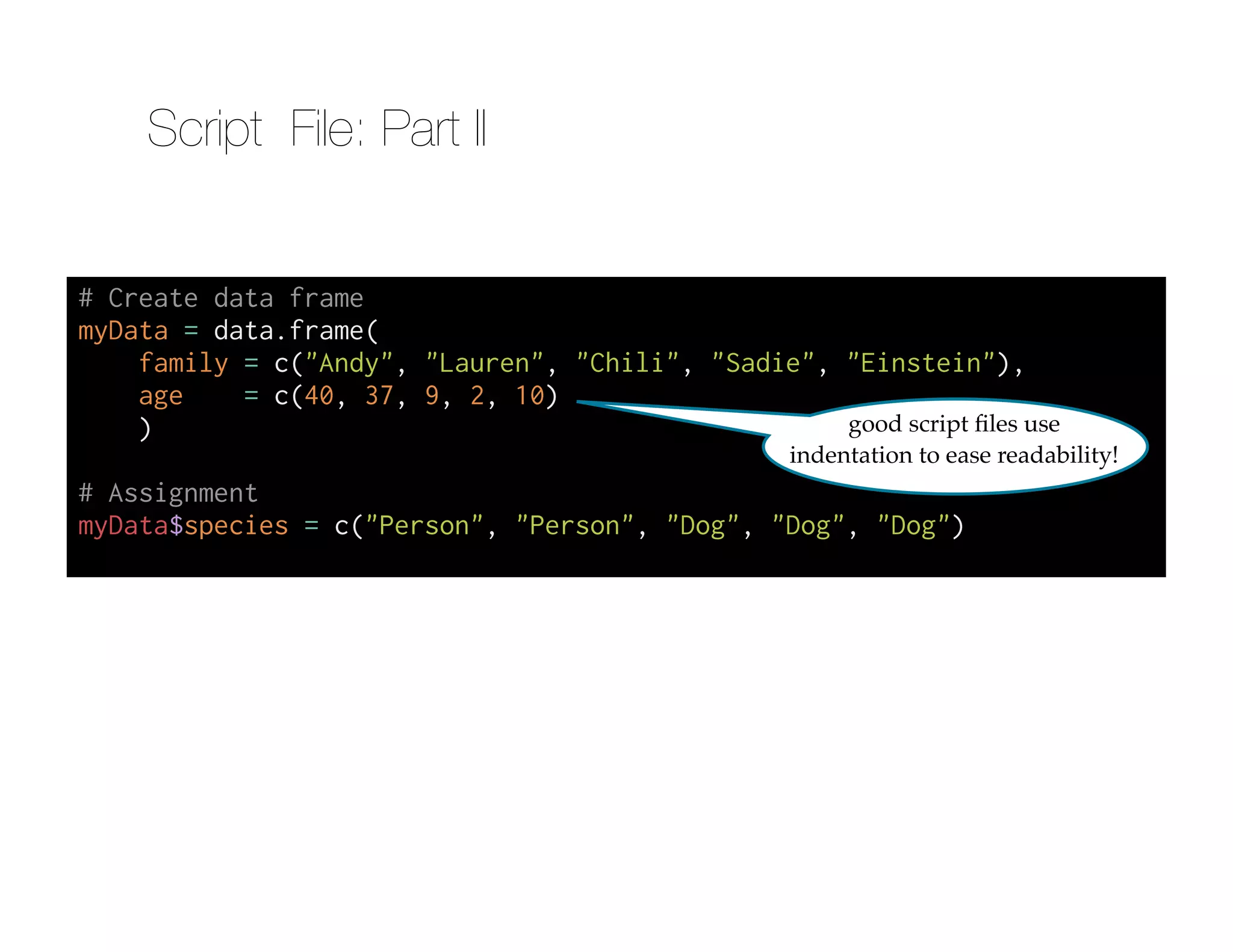
# Create data frame
myData = data.frame(
family = c("Andy", "Lauren", "Chili", "Sadie", "Einstein"),
age = c(40, 37, 9, 2, 10)
)
!
# Assignment
myData$species = c("Person", "Person", "Dog", "Dog", "Dog")
good script files use
indentation to ease readability!
Script File: Part II
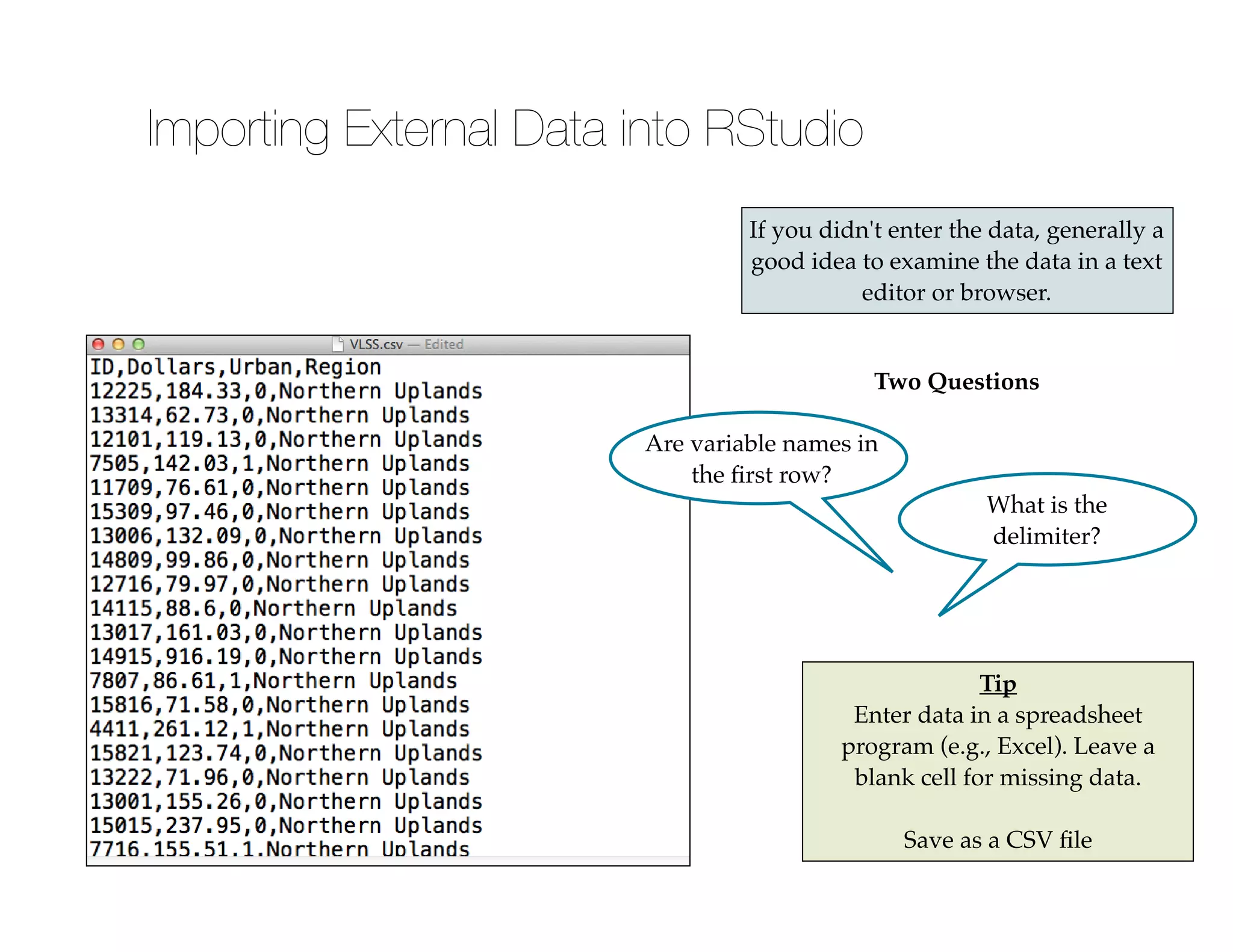
If you didn't enter the data, generally a
good idea to examine the data in a text
editor or browser.
Two Questions
Are variable names in
the first row?
What is the
delimiter?
Tip!
Enter data in a spreadsheet
program (e.g., Excel). Leave a
blank cell for missing data.!
!
Save as a CSV file
Importing External Data into RStudio
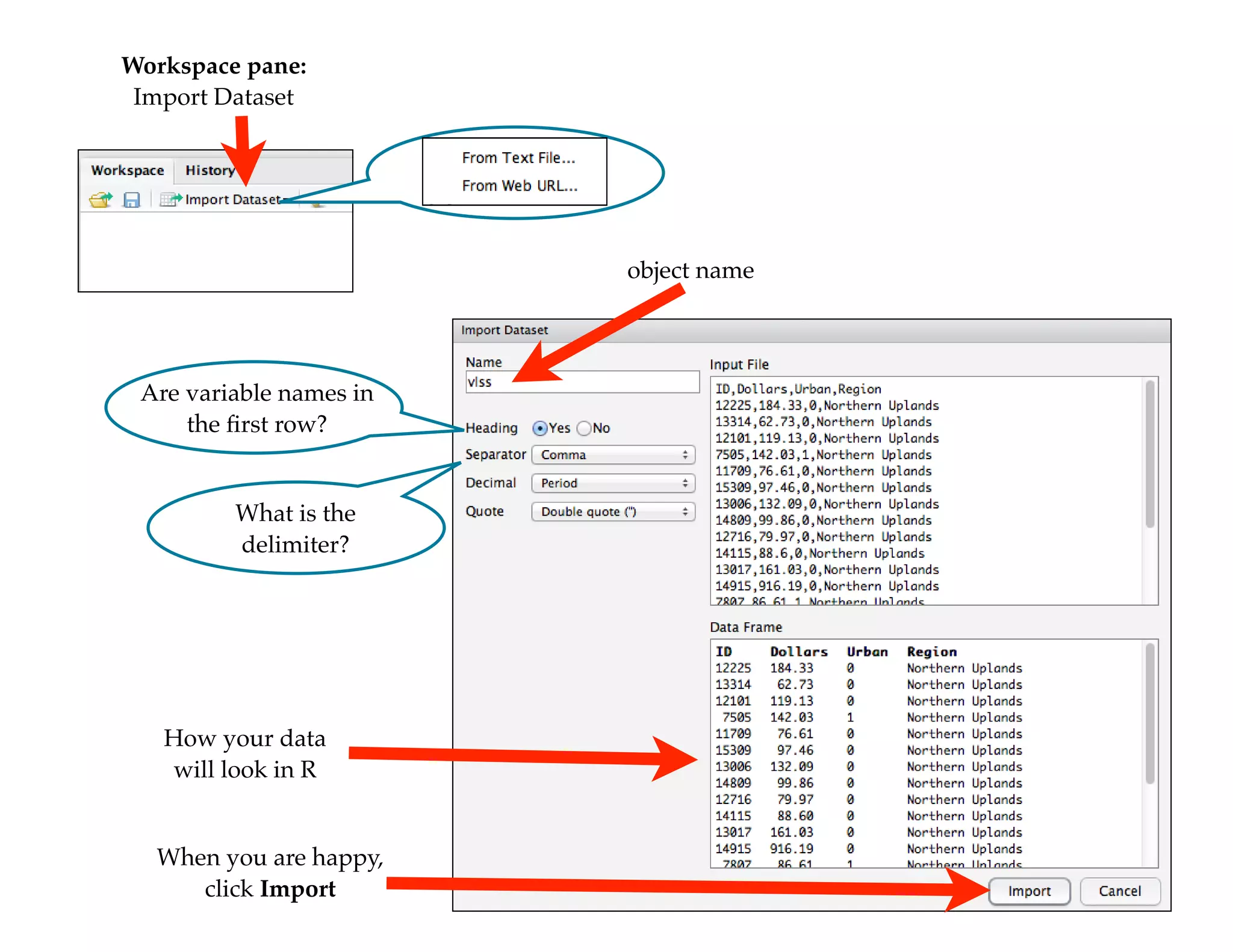
object name
How your data
will look in R
When you are happy,
click Import
Are variable names in
the first row?
What is the
delimiter?
Workspace pane:
Import Dataset
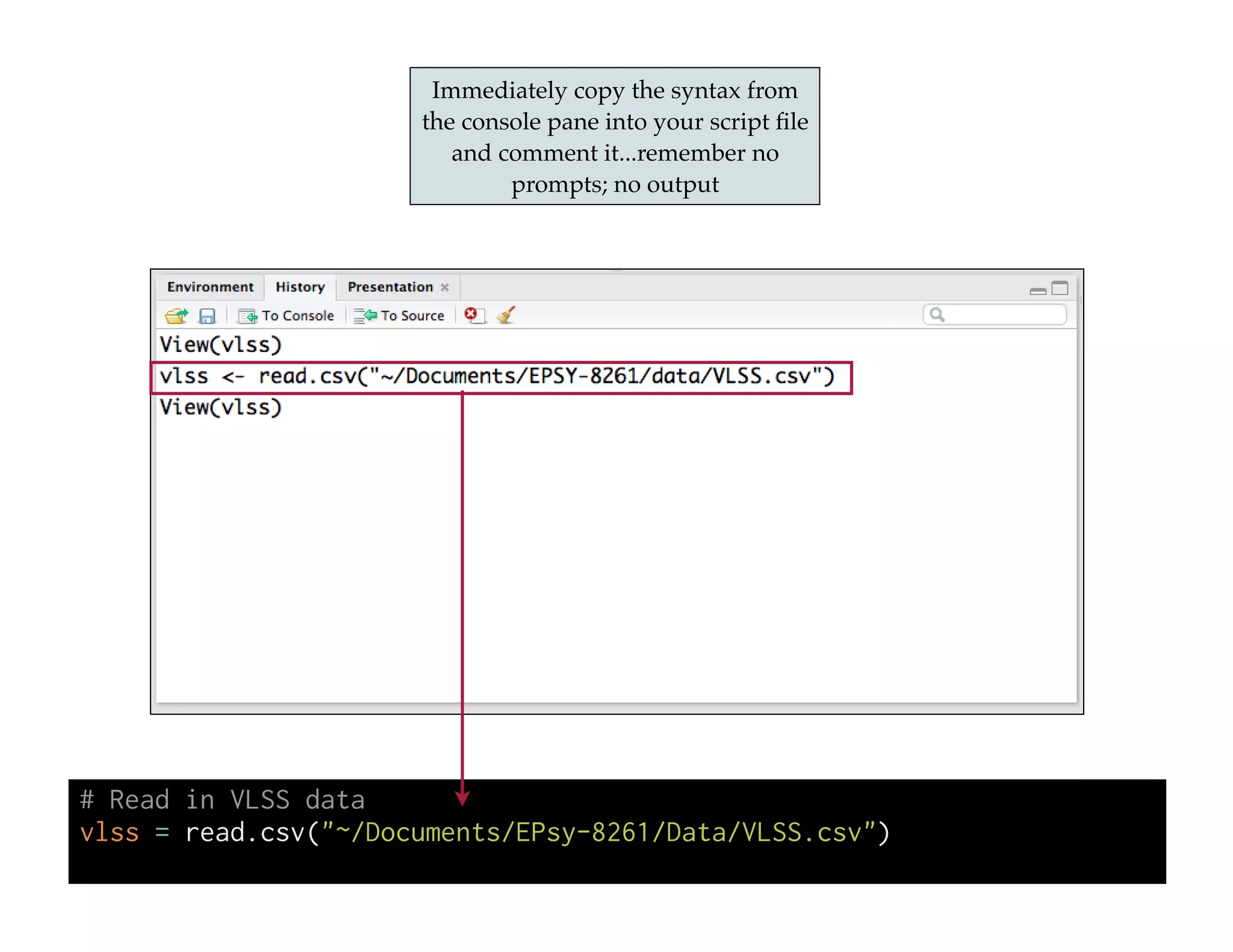
Immediately copy the syntax from
the console pane into your script file
and comment it...remember no
prompts; no output
# Read in VLSS data
vlss = read.csv("~/Documents/EPsy-8261/Data/VLSS.csv")
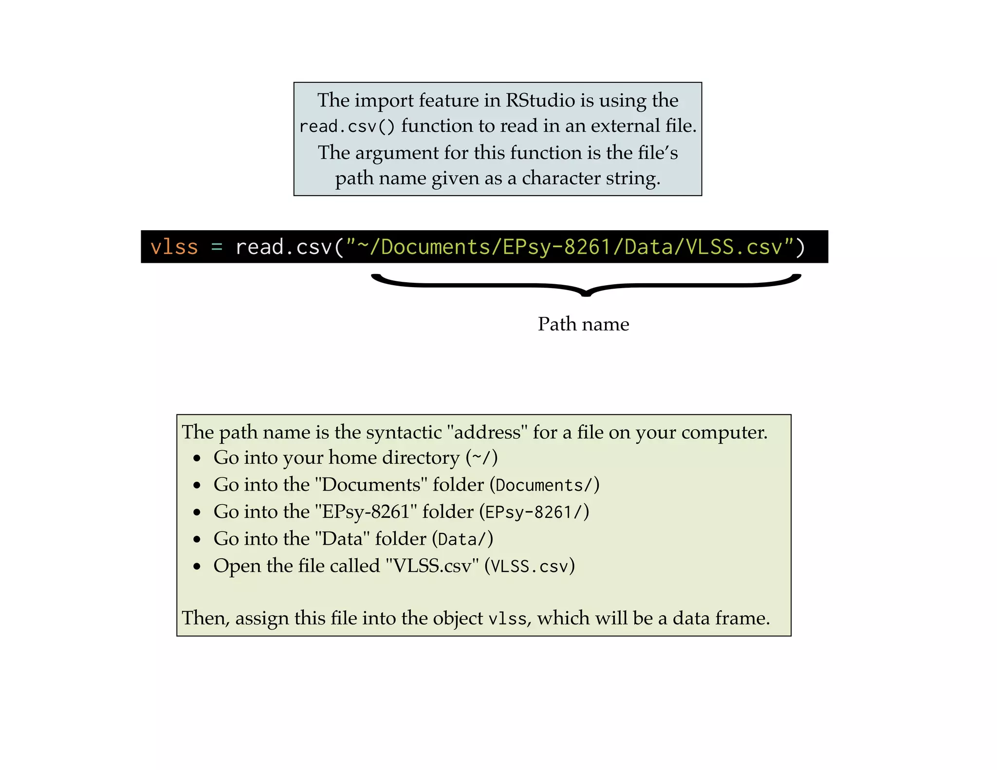
The path name is the syntactic "address" for a file on your computer.!
• Go into your home directory (~/)!
• Go into the "Documents" folder (Documents/)!
• Go into the "EPsy-8261" folder (EPsy-8261/) !
• Go into the "Data" folder (Data/)!
• Open the file called "VLSS.csv" (VLSS.csv)!
!
Then, assign this file into the object vlss, which will be a data frame.
{
Path name
vlss = read.csv("~/Documents/EPsy-8261/Data/VLSS.csv")
The import feature in RStudio is using the
read.csv() function to read in an external file.
The argument for this function is the file’s
path name given as a character string.
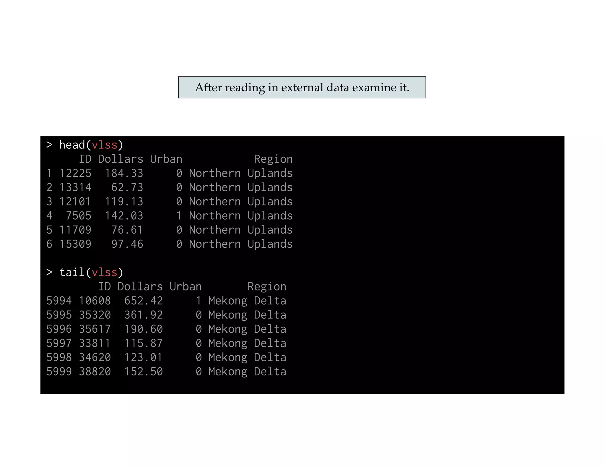
After reading in external data examine it.
> head(vlss)
ID Dollars Urban Region
1 12225 184.33 0 Northern Uplands
2 13314 62.73 0 Northern Uplands
3 12101 119.13 0 Northern Uplands
4 7505 142.03 1 Northern Uplands
5 11709 76.61 0 Northern Uplands
6 15309 97.46 0 Northern Uplands
!
> tail(vlss)
ID Dollars Urban Region
5994 10608 652.42 1 Mekong Delta
5995 35320 361.92 0 Mekong Delta
5996 35617 190.60 0 Mekong Delta
5997 33811 115.87 0 Mekong Delta
5998 34620 123.01 0 Mekong Delta
5999 38820 152.50 0 Mekong Delta
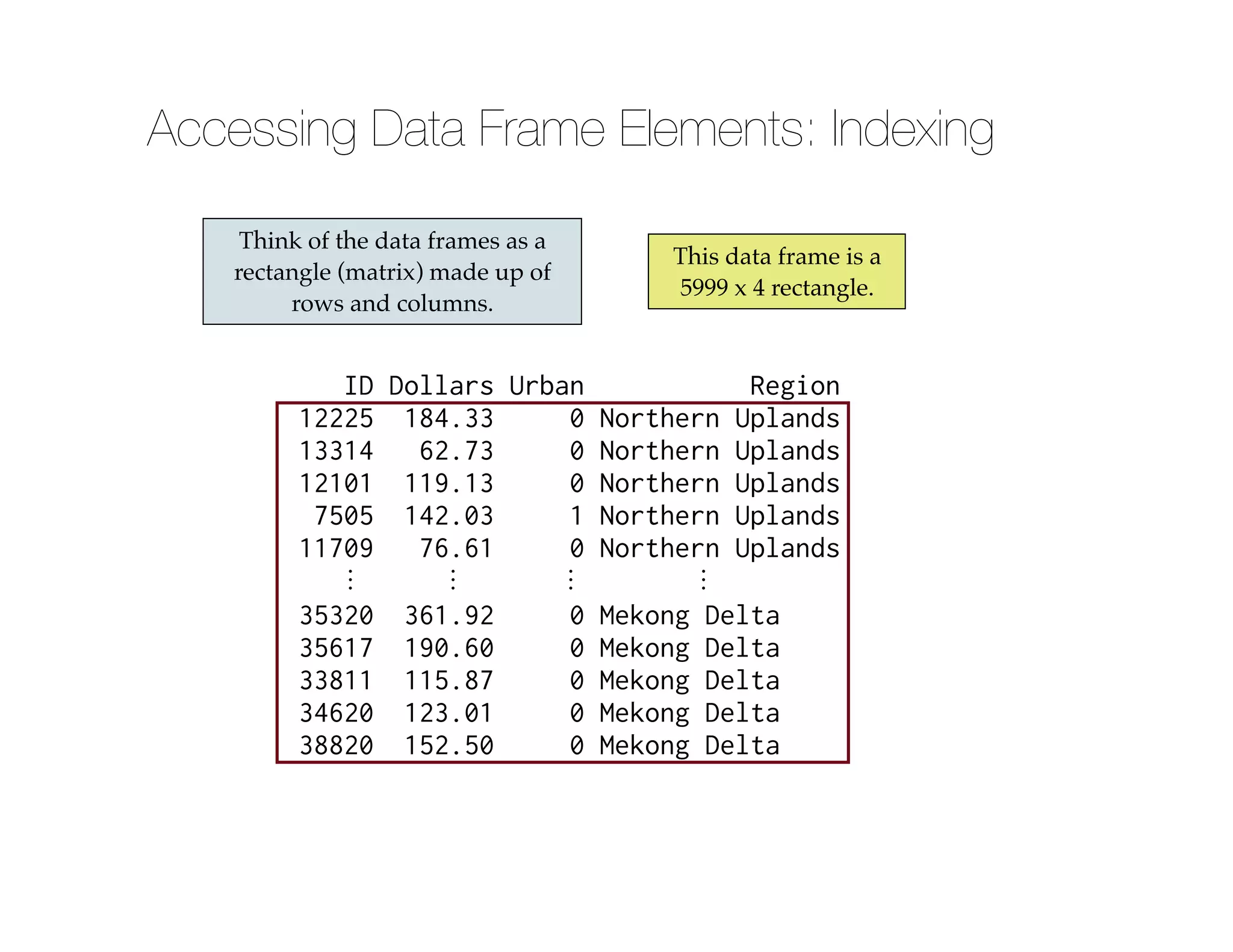
Think of the data frames as a
rectangle (matrix) made up of
rows and columns.
ID Dollars Urban Region
12225 184.33 0 Northern Uplands
13314 62.73 0 Northern Uplands
12101 119.13 0 Northern Uplands
7505 142.03 1 Northern Uplands
11709 76.61 0 Northern Uplands
⋮ ⋮ ⋮ ⋮
35320 361.92 0 Mekong Delta
35617 190.60 0 Mekong Delta
33811 115.87 0 Mekong Delta
34620 123.01 0 Mekong Delta
38820 152.50 0 Mekong Delta
This data frame is a
5999 x 4 rectangle.
Accessing Data Frame Elements: Indexing
> vlss[3, 1]
[1] 12101
!
> vlss[1, 3]
[1] 0
!
> vlss[1, ]
child age toddler
1 Andy 1 FALSE
!
> myData[1, ]
ID Dollars Urban Region
1 12225 184.33 0 Northern Uplands
This is the ID for the 3rd subject.!
(3rd row, 1st column)
Omitting the row or column gives
all the elements of the omitted part
of the “address”. In this case all
columns in the 1st row
To access elements we give the “address”
of the element within the rectangle, [row,
column]. This is called indexing.
This is Urban value for the 1st
subject.!
(1st row, 3rd column)
> vlss[ , 2]
[Output not shown]
!
> vlss$Dollars
[Output not shown]
!
> myData[[2]]
[Output not shown]
!
> mean(vlss$Dollars)
[1] 212.5778
You can also access columns by using
the variable names and $ operator.!
dataframe$variable
You can also use list indexing,
double square brackets.
Accessing Variables (columns)
> age
[1] 40 37 9 2 10
!
> age[2]
[1] 37
!
> myData$age[2]
[1] 37
!
> myData[[2]][2]
[1] 37
Indexing also works on vectors.
Since vectors only have one
dimension, we only need to provide
a single value in the “address”
Indexing a Vector
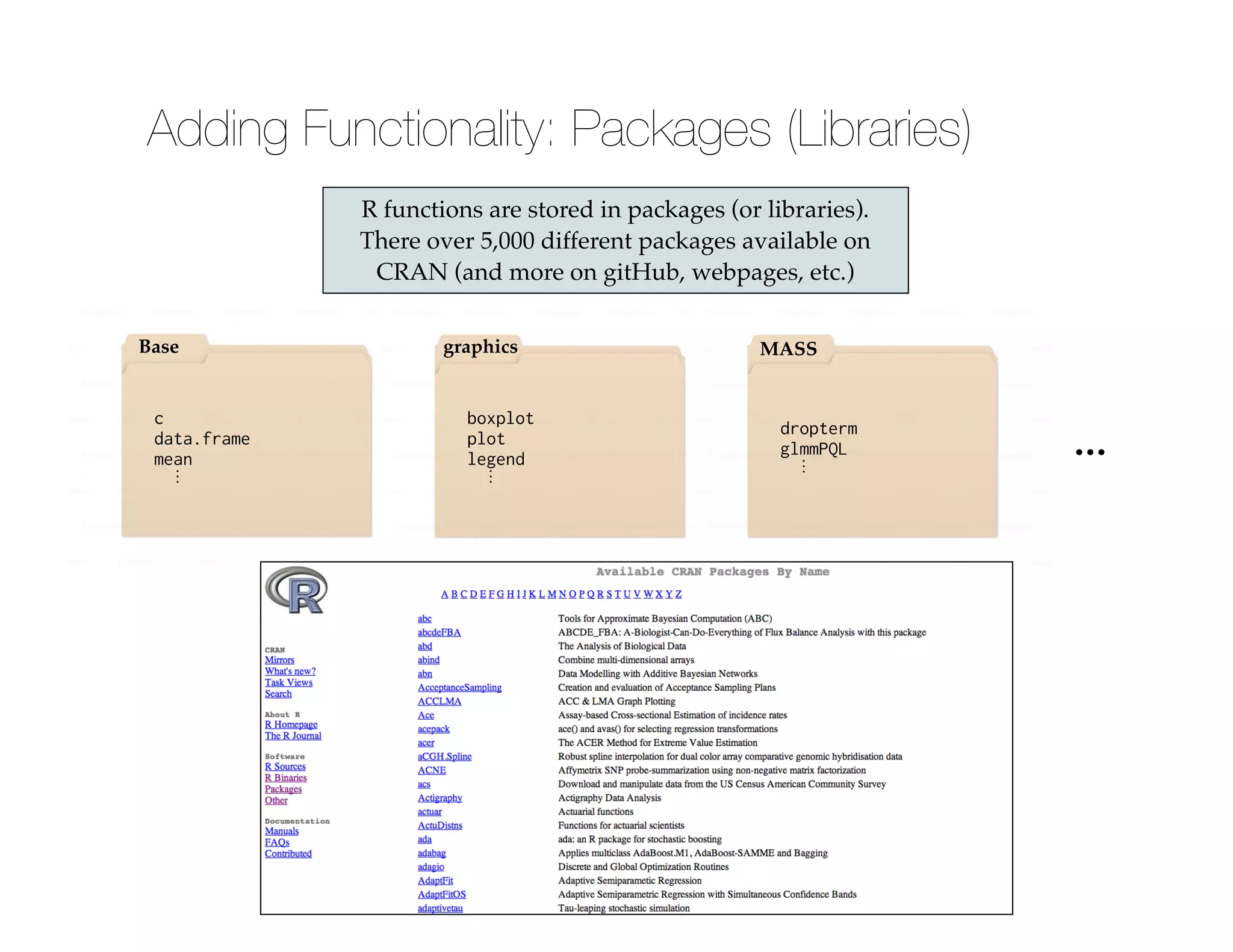
R functions are stored in packages (or libraries).
There over 5,000 different packages available on
CRAN (and more on gitHub, webpages, etc.)
c
data.frame
mean
⋮
Base
boxplot
plot
legend
⋮
graphics
dropterm
glmmPQL
⋮
MASS
...
Adding Functionality: Packages (Libraries)
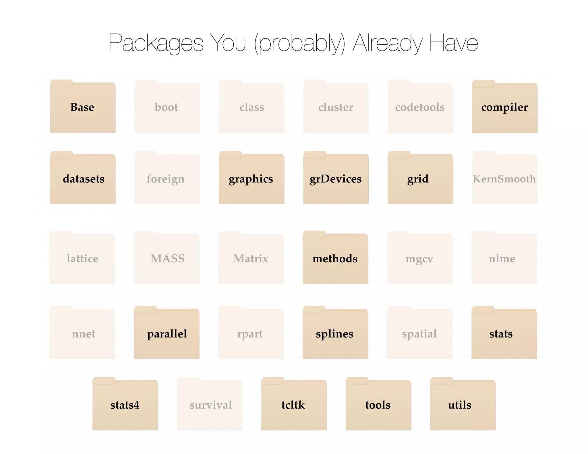
Base boot class cluster codetools compiler
datasets foreign graphics grDevices grid KernSmooth
lattice MASS Matrix methods mgcv nlme
nnet parallel rpart splines spatial stats
stats4 survival tcltk tools utils
Packages You (probably) Already Have
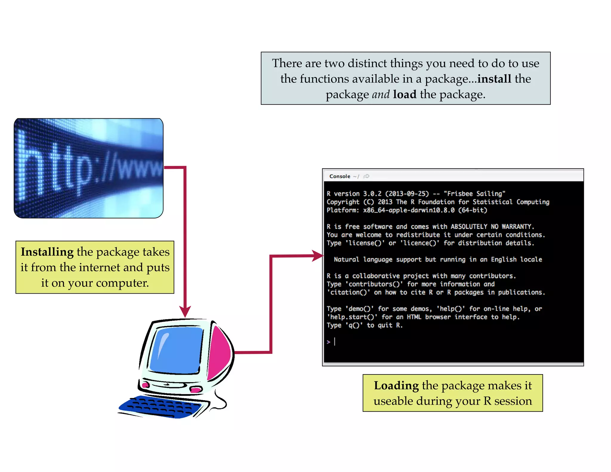
There are two distinct things you need to do to use
the functions available in a package...install the
package and load the package.
Installing the package takes
it from the internet and puts
it on your computer.
Loading the package makes it
useable during your R session
Loading Packages that are Installed
> library(MASS)
!
> library(survival)
Loading required package: splines
The library() function is used to load packages
that have previously been installed.
Some packages requires other packages
(dependencies) to work. For example, the
survival package is dependent on the splines
package.
Packages will need to be loaded every time
you launch a new R session.
Once the package is loaded, all of the
functions, data sets, etc. in that
package are available to you.
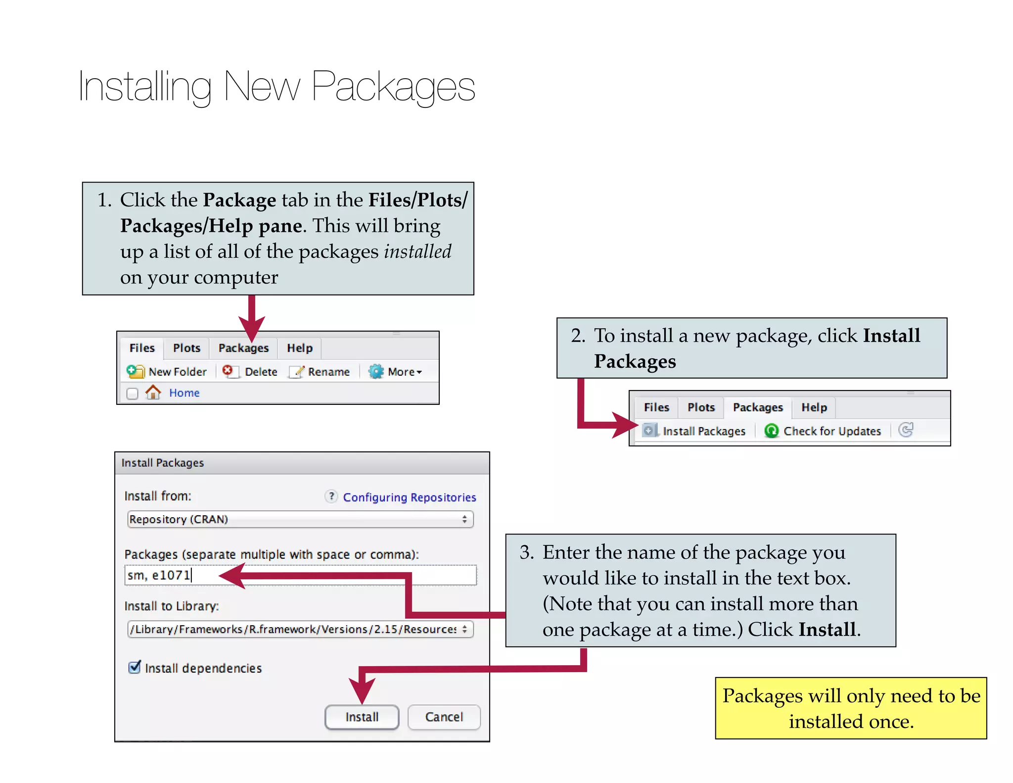
2. To install a new package, click Install
Packages
1. Click the Package tab in the Files/Plots/
Packages/Help pane. This will bring
up a list of all of the packages installed
on your computer
3. Enter the name of the package you
would like to install in the text box.
(Note that you can install more than
one package at a time.) Click Install.
Installing New Packages
Packages will only need to be
installed once.

Introduction to R

  • 1.
  • 2.
    Some Things toRemember... • R is case-sensitive anova is different than Anova is different than ANOVA • R does exactly what the user codes • R has a "long-term" memory... The user and R often don’t see “eye-to-eye” ...but only in the current session
  • 3.
    RStudio Console pane: Interactivetyping Script pane: non-interactive typing
  • 4.
    > Console Pane (Interactive) Rprompt...R is waiting for a command > 3 + 2 ! [1] 5 After inputting a command hit <enter> R returned value...the brackets indicate the ith returned element.! Here they indicate the first returned element.! (They can be ignored for now (we are more interested in the returned value of 5.) > 3 + ! + Continuation prompt... The previous command was not properly ended prior to hitting <enter>! ! • Finish command! • Hit <esc> until you get the command prompt again. Then re-try {Two options
  • 5.
    > 4 *5 [1] 20 ! > 10 ^ 3 [1] 1000 ! > 1 / 0 [1] Inf Space is for humans. > 4 * 5 > 4*5 > 4 *5 are all the same to R
  • 6.
    > sqrt(100) [1] 10 ! >log(7) [1] 1.94591 ! > sin(50) [1] -0.2623749 ! > exp(3) [1] 20.08554 ! > log(100, 10) [1] 2 ! > log(100, base = 10) [1] 2 Three components! • Function! • Argument! • Returned value Arguments! Enclosed in parentheses Multiple arguments separated by commas Can be named or unnamed Computations in R using Functions
  • 7.
    > log(100, 10) [1]2 ! > log(10, 100) [1] 0.5 ! > log(x = 100, base = 10) [1] 2 ! > log(base = 10, x = 100) [1] 2 ! > log(100, base = 10) [1] 2 Order does not matter for named arguments Conventionally, the first argument is often unnamed and the remainder are named Order matters for unnamed arguments
  • 8.
    Connecting Computations inR Two methods of connecting computations ! • Chaining! • Assignment ! > sqrt( log(100, base = 10) ) ! [1] 1.414214 ! > chili <- log(100, base = 10) > chili = log(100, base = 10) ! > sqrt(chili) [1] 1.414214 Chaining uses a complete computation as the argument for another computation. Assignment stores the returned value from a computation as a named object. The assignment operator is either <- or =
  • 9.
    > chili =3 ! > sqrt(chili) [1] 1.732051 ! > chili [1] 3 When an object name is re-used, the previous value of the object is lost. Workspace: List of current objects • Pretty much any name can be used! • Descriptive is better! ‣ chili is not a good object name! • Names cannot include hyphens or spaces! • Names cannot begin with a digit! • Conventions in CS! ‣ myData (bumpy/camel-case)! ‣ my_data (use underscore/period) Objects
  • 10.
    Saving Your Work:Script Files Record syntax in a script file • Includes syntax (R commands) only! ‣ No prompts! ‣ No output! • Should also include comments! ‣ # indicates a comment
  • 11.
    # Arithmetic computations 3+ 2 4 * 5 10 ^ 3 ! # Assignment chili = log(100, base = 10) ! # Compute things sqrt(chili) # Find the square root log(chili) # Find the natural logarithm good script files have comments Comments can also be placed on an existing line Syntax in the script file can be executed by highlighting it and pressing the Run button! !
  • 12.
    Vectors are collectionsof data (univariate; a single variable). They are typically assigned to an object. To create a vector use the c() function. > age = c(40, 37, 9, 2, 10) ! > age [1] 40 37 9 2 10 ! > age + 5 [1] 45 42 14 7 15 ! > age ^ 2 [1] 1600 1369 81 4 100 ! > mean(age) [1] 19.6 ! > sum(age) [1] 98 Some computations are element-wise Some computations are vector-wise Data Structures: Vectors
  • 13.
    Not all vectorsare numeric. R has six different types of vectors. Use class() to find out what type you have. > family = c("Andy", "Lauren", "Chili", "Sadie", "Einstein") ! > family [1] "Andy" "Lauren" "Chili" "Sadie" "Einstein" ! > family + 5 Error in family + 5 : non-numeric argument to binary operator ! > length(family) [1] 5 ! > family2 = c("Andy", "Lauren", "Chili", 1, 5) ! > family2 [1] "Andy" "Lauren" "Chili" "1" "5" In a character vector (a.k.a. strings, literals) each element is a character string. Character strings are delimited by quotation marks. All elements in a vector have to be of the same type...if not they will be coerced to the same type Character Vectors
  • 14.
    > myLogical =c(TRUE, FALSE, FALSE) ! > age [1] 40 37 9 2 10 ! > age > 10 [1] TRUE TRUE FALSE FALSE FALSE ! > people = (age > 10) ! > length(people) [1] 5 ! > people + 1 [1] 2 2 1 1 1 In a logical vector each element is TRUE or FALSE. Logical elements are not delimited by quotation marks. Logical vectors are often generated through conditional statements Logical elements have numeric values associated with them, namely 0 (FALSE) or 1 (TRUE). Logical Vectors
  • 15.
    Data frames havea tabular (rectangular) structure made up of rows (cases) and columns (variables).! • Columns need to have the same length! • Columns can be of different vector types! • Columns have names family age people Andy 40 TRUE Lauren 37 TRUE Chili 9 FALSE Sadie 2 FALSE Einstein 10 FALSE }Same length Names Data Structures: Data Frames
  • 16.
    > myData =data.frame(family, age, people) ! > myData family age people 1 Andy 1 FALSE 2 Lauren 6 TRUE 3 Chili 7 TRUE 4 Mojo 7 TRUE 5 Einstein 10 TRUE You can create data frames by binding together existing vectors. Creating Data Frames
  • 17.
    > myData =data.frame( family = c("Andy", "Lauren", "Chili", "Sadie", "Einstein"), age = c(40, 37, 9, 2, 10) ) ! > myData family age 1 Andy 40 2 Lauren 37 3 Chili 9 4 Sadie 2 5 Einstein 10 ! > myData$species = c("Person", "Person", "Dog", "Dog", "Dog") ! > myData family age species 1 Andy 40 Person 2 Lauren 37 Person 3 Chili 9 Dog 4 Sadie 2 Dog 5 Einstein 10 Dog Data frames can also be created from scratch. New variables can be appended to existing data frames using the $ operator.
  • 18.
    # Create dataframe myData = data.frame( family = c("Andy", "Lauren", "Chili", "Sadie", "Einstein"), age = c(40, 37, 9, 2, 10) ) ! # Assignment myData$species = c("Person", "Person", "Dog", "Dog", "Dog") good script files use indentation to ease readability! Script File: Part II
  • 19.
    If you didn'tenter the data, generally a good idea to examine the data in a text editor or browser. Two Questions Are variable names in the first row? What is the delimiter? Tip! Enter data in a spreadsheet program (e.g., Excel). Leave a blank cell for missing data.! ! Save as a CSV file Importing External Data into RStudio
  • 20.
    object name How yourdata will look in R When you are happy, click Import Are variable names in the first row? What is the delimiter? Workspace pane: Import Dataset
  • 21.
    Immediately copy thesyntax from the console pane into your script file and comment it...remember no prompts; no output # Read in VLSS data vlss = read.csv("~/Documents/EPsy-8261/Data/VLSS.csv")
  • 22.
    The path nameis the syntactic "address" for a file on your computer.! • Go into your home directory (~/)! • Go into the "Documents" folder (Documents/)! • Go into the "EPsy-8261" folder (EPsy-8261/) ! • Go into the "Data" folder (Data/)! • Open the file called "VLSS.csv" (VLSS.csv)! ! Then, assign this file into the object vlss, which will be a data frame. { Path name vlss = read.csv("~/Documents/EPsy-8261/Data/VLSS.csv") The import feature in RStudio is using the read.csv() function to read in an external file. The argument for this function is the file’s path name given as a character string.
  • 23.
    After reading inexternal data examine it. > head(vlss) ID Dollars Urban Region 1 12225 184.33 0 Northern Uplands 2 13314 62.73 0 Northern Uplands 3 12101 119.13 0 Northern Uplands 4 7505 142.03 1 Northern Uplands 5 11709 76.61 0 Northern Uplands 6 15309 97.46 0 Northern Uplands ! > tail(vlss) ID Dollars Urban Region 5994 10608 652.42 1 Mekong Delta 5995 35320 361.92 0 Mekong Delta 5996 35617 190.60 0 Mekong Delta 5997 33811 115.87 0 Mekong Delta 5998 34620 123.01 0 Mekong Delta 5999 38820 152.50 0 Mekong Delta
  • 24.
    Think of thedata frames as a rectangle (matrix) made up of rows and columns. ID Dollars Urban Region 12225 184.33 0 Northern Uplands 13314 62.73 0 Northern Uplands 12101 119.13 0 Northern Uplands 7505 142.03 1 Northern Uplands 11709 76.61 0 Northern Uplands ⋮ ⋮ ⋮ ⋮ 35320 361.92 0 Mekong Delta 35617 190.60 0 Mekong Delta 33811 115.87 0 Mekong Delta 34620 123.01 0 Mekong Delta 38820 152.50 0 Mekong Delta This data frame is a 5999 x 4 rectangle. Accessing Data Frame Elements: Indexing
  • 25.
    > vlss[3, 1] [1]12101 ! > vlss[1, 3] [1] 0 ! > vlss[1, ] child age toddler 1 Andy 1 FALSE ! > myData[1, ] ID Dollars Urban Region 1 12225 184.33 0 Northern Uplands This is the ID for the 3rd subject.! (3rd row, 1st column) Omitting the row or column gives all the elements of the omitted part of the “address”. In this case all columns in the 1st row To access elements we give the “address” of the element within the rectangle, [row, column]. This is called indexing. This is Urban value for the 1st subject.! (1st row, 3rd column)
  • 26.
    > vlss[ ,2] [Output not shown] ! > vlss$Dollars [Output not shown] ! > myData[[2]] [Output not shown] ! > mean(vlss$Dollars) [1] 212.5778 You can also access columns by using the variable names and $ operator.! dataframe$variable You can also use list indexing, double square brackets. Accessing Variables (columns)
  • 27.
    > age [1] 4037 9 2 10 ! > age[2] [1] 37 ! > myData$age[2] [1] 37 ! > myData[[2]][2] [1] 37 Indexing also works on vectors. Since vectors only have one dimension, we only need to provide a single value in the “address” Indexing a Vector
  • 28.
    R functions arestored in packages (or libraries). There over 5,000 different packages available on CRAN (and more on gitHub, webpages, etc.) c data.frame mean ⋮ Base boxplot plot legend ⋮ graphics dropterm glmmPQL ⋮ MASS ... Adding Functionality: Packages (Libraries)
  • 29.
    Base boot classcluster codetools compiler datasets foreign graphics grDevices grid KernSmooth lattice MASS Matrix methods mgcv nlme nnet parallel rpart splines spatial stats stats4 survival tcltk tools utils Packages You (probably) Already Have
  • 30.
    There are twodistinct things you need to do to use the functions available in a package...install the package and load the package. Installing the package takes it from the internet and puts it on your computer. Loading the package makes it useable during your R session
  • 31.
    Loading Packages thatare Installed > library(MASS) ! > library(survival) Loading required package: splines The library() function is used to load packages that have previously been installed. Some packages requires other packages (dependencies) to work. For example, the survival package is dependent on the splines package. Packages will need to be loaded every time you launch a new R session. Once the package is loaded, all of the functions, data sets, etc. in that package are available to you.
  • 32.
    2. To installa new package, click Install Packages 1. Click the Package tab in the Files/Plots/ Packages/Help pane. This will bring up a list of all of the packages installed on your computer 3. Enter the name of the package you would like to install in the text box. (Note that you can install more than one package at a time.) Click Install. Installing New Packages Packages will only need to be installed once.