2
Basics & Distributionof Data
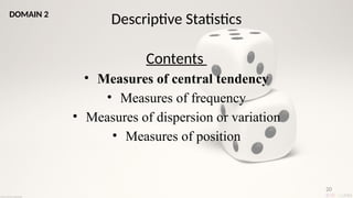
Contents
• Introduction
• Application and uses
• Limitations
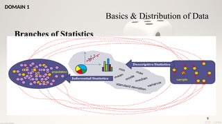
• Branches
• Data
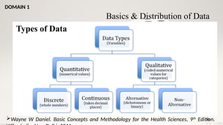
• Types
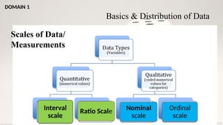
• Scales
• Collection
• Presentation
DOMAIN 1
3.
3
Basics & Distributionof Data
Introduction
– Statistics defined as the science of
Collection,
organisation,
presentation,
analysis and
interpretation of numerical data.”
Concise definition by Croxton and Cowden
DOMAIN 1
5
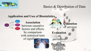
Application and Usesof Biostatistics
Association
between causative
factors and effects
by comparison
with statistical tests
of significance
Evaluation
of
preventive
and
therapeutic
strategies
Utilization
of services
Prediction
of events
Basics & Distribution of Data
DOMAIN 1
6.
6
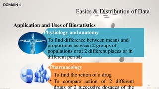
Application and Usesof Biostatistics
Physiology and anatomy
• To find difference between means and
proportions between 2 groups of
populations or at 2 different places or in
different periods
Pharmacology
• To find the action of a drug
• To compare action of 2 different
drugs or 2 successive dosages of the
Basics & Distribution of Data
DOMAIN 1
7.
7
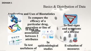
Application and Usesof Biostatistics
To compare the
efficacy of a
particular drug,
operation or line of
treatment
To find an
association
between 2
attributes
To find signs
and symptoms
of a disease
To test
usefulness of
In
epidemiological
studies
Evaluation of
measures
Basics & Distribution of Data
DOMAIN 1
8.
8
Limitations of statisticsin health science
How representative is your sample?
How well the statistics is suited to the study of qualitative
phenomena?
Statistics does not study individuals
Statistical Laws are not exact
Basics & Distribution of Data
DOMAIN 1
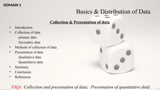
12
Collection & Presentationof data
• Introduction
• Collection of data
primary data
Secondary data
• Methods of collection of data
• Presentation of data
Qualitative data
Quantitative data
• Summary
• Conclusion
• References
FAQs: Collection and presentation of data; Presentation of quantitative data
Basics & Distribution of Data
DOMAIN 1
13.
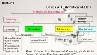
Methods of datacollection
Secondary
Sources
Primary
Sources
Documents
oGovt publications
oEarlier research
oCensus
oPersonal records
oClient histories
oService records
Observation
Participant
Non-participant
Interviewing
Structured
Unstructured
Questionnaire
Mailed
Collective
Basics & Distribution of Data
Wayne W Daniel. Basic Concepts and Methodology for the Health
Sciences, 9th
Edition. Wiley India. New Delhi; 2011.
DOMAIN 1
13
14.
14
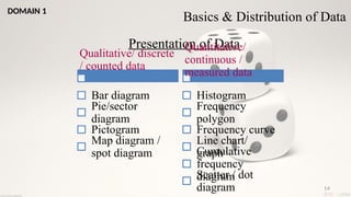
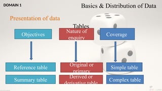
Presentation of Data
Qualitative/discrete
/ counted data
Bar diagram
Pie/sector
diagram
Pictogram
Map diagram /
spot diagram
Quantitative/
continuous /
measured data
Histogram
Frequency
polygon
Frequency curve
Line chart/
graph
Cumulative
frequency
diagram
Scatter / dot
diagram
Basics & Distribution of Data
DOMAIN 1
15.
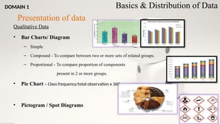
Qualitative Data
• BarCharts/ Diagram
– Simple
– Compound - To compare between two or more sets of related groups.
– Proportional - To compare proportion of components
present in 2 or more groups.
• Pie Chart - Class frequency/total observation x 360
• Pictogram / Spot Diagrams
15
Presentation of data
Basics & Distribution of Data
DOMAIN 1
18
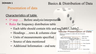
Characteristics of table
•1st
step ….. Before analysis/interpretation
• Rules for frequency distribution table
– Each table should contain title and no-Table1,Table2….
– Headings …rows & columns clear n concise
– Units of measurements specified
– Source of data mentioned
– Additional Information - end note
Presentation of data
Basics & Distribution of Data
DOMAIN 1
19.
19
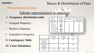
Tabular representation instatistics
I. Frequency distribution table
• Grouped frequency
• Relative frequency
• Cumulative frequency
II. Contingency Table
III. Cross Tabulation
Presentation of data
Basics & Distribution of Data
DOMAIN 1
21
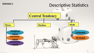
Central Tendency
Mean MedianMode
Weighted
mean
Harmonic
mean
Geometric
mean
Descriptive Statistics
DOMAIN 2
Unimodal
Bi Modal
22.
22
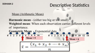
Mean (Arithmetic Mean)
01 2 3 4 5 6 7 8 9 10 0 1 2 3 4 5 6 7 8 9 10 12 14
Mean = 5 Mean = 6
Descriptive Statistics
DOMAIN 2
Harmonic mean - (either too big or too small)
Weighted mean: When each observation carries different levels
of importance.
Geometric Mean - Exponential data
23.
23
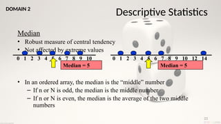
Median
• Robust measureof central tendency
• Not affected by extreme values
• In an ordered array, the median is the “middle” number
– If n or N is odd, the median is the middle number
– If n or N is even, the median is the average of the two middle
numbers
0 1 2 3 4 5 6 7 8 9 10 0 1 2 3 4 5 6 7 8 9 10 12 14
Median = 5 Median = 5
Descriptive Statistics
DOMAIN 2
24.
24
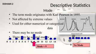
Mode
• The termmode originates with Karl Pearson in 1895.
• Not affected by extreme values
• Used for either numerical or categorical
data
• There may be no mode
• There may be several modes
0 1 2 3 4 5 6 7 8 9 10 11 12 13 14
Mode = 9
0 1 2 3 4 5 6
No Mode
Descriptive Statistics
DOMAIN 2
25.
25
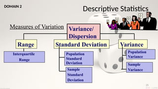
Measures of VariationVariance/
Dispersion
Variance
Standard Deviation
Population
Variance
Sample
Variance
Population
Standard
Deviation
Sample
Standard
Deviation
Range
Interquartile
Range
Descriptive Statistics
DOMAIN 2
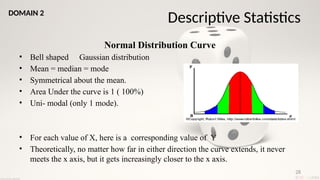
28
Normal Distribution Curve
•Bell shaped Gaussian distribution
• Mean = median = mode
• Symmetrical about the mean.
• Area Under the curve is 1 ( 100%)
• Uni- modal (only 1 mode).
• For each value of X, here is a corresponding value of Y
• Theoretically, no matter how far in either direction the curve extends, it never
meets the x axis, but it gets increasingly closer to the x axis.
Descriptive Statistics
DOMAIN 2
29.
29
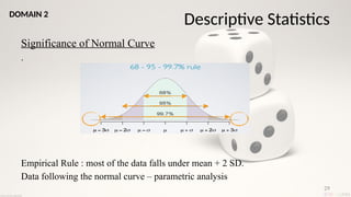
Significance of NormalCurve
.
Empirical Rule : most of the data falls under mean + 2 SD.
Data following the normal curve – parametric analysis
Descriptive Statistics
DOMAIN 2
30.
30
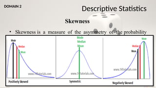
Skewness
• Skewness isa measure of the asymmetry of the probability
distribution about its mean.
Descriptive Statistics
DOMAIN 2
31.
31
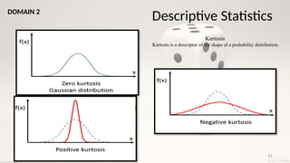
Kurtosis
Kurtosis is adescriptor of the shape of a probability distribution.
Descriptive Statistics
DOMAIN 2
35
Introduction & Rationaleof Hypothesis Testing
• It is considered as one of the principal instrument in the
research
• A statistical procedure by which one can conclude if the observed
results from the sample is due to chance or not.
• In social science, it enables us to make probability statement and
generalization to the population.
DOMAIN 3
36.
38
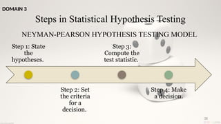
Steps in StatisticalHypothesis Testing
NEYMAN-PEARSON HYPOTHESIS TESTING MODEL
Step 1: State
the
hypotheses.
Step 2: Set
the criteria
for a
decision.
Step 3:
Compute the
test statistic.
Step 4: Make
a decision.
DOMAIN 3
37.
39
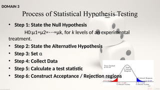
Non
Critical
Region
Critical Region CriticalRegion
Critical Value Critical Value
Two-Tailed
CV=-1.65 CV=1.65
α=0.10
α/2=0.05
α/2=0.05
Process of Statistical Hypothesis Testing
• Step 1: State the Null Hypothesis
H0:μ1=μ2= =μ
⋯ k, for k levels of an experimental
treatment.
• Step 2: State the Alternative Hypothesis
• Step 3: Set α
• Step 4: Collect Data
• Step 5: Calculate a test statistic
• Step 6: Construct Acceptance / Rejection regions
DOMAIN 3
38.
40
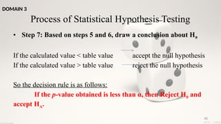
• Step 7:Based on steps 5 and 6, draw a conclusion about H0
If the calculated value < table value accept the null hypothesis
If the calculated value > table value reject the null hypothesis
So the decision rule is as follows:
If the p-value obtained is less than α, then Reject H0 and
accept HA.
Process of Statistical Hypothesis Testing
DOMAIN 3
39.
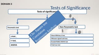
Tests of significance
Parametrictest Non Parametric test
z-test ,
t- test,
ANOVA
Mann-Whitney U test,
Wilcoxon signed rank test,
Kruskal-Wallis ANOVA test
Fried man test
Tests of Significance
Chi- Square test
Correlation
RegressionAnalysis
DOMAIN 3
40.
42
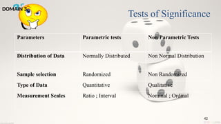
Parameters Parametric testsNon Parametric Tests
Distribution of Data Normally Distributed Non Normal Distribution
Sample selection Randomized Non Randomized
Type of Data Quantitative Qualitative
Measurement Scales Ratio ; Interval Nominal ; Ordinal
Tests of Significance
DOMAIN 3
41.
45
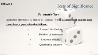
Parametric Tests
Parametric statisticsis a branch of statistics which assumes that sample data
comes from a population that follows:
• A normal distribution
• Fixed set of parameters
• Randomly selected
• Quantitative in nature
Tests of Significance
DOMAIN 3
47
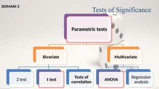
Parametric tests
Bivariate
Z testt test
Tests of
correlati
on
Multivariate
ANOVA
Regressio
n
analysis
Tests of Significance
DOMAIN 3
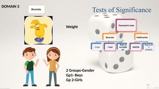
Bivariate
Weight
2 Groups-Gender
Gp1- Boys
Gp 2-Girls
44.
48
Parametric tests
Bivariate
Z testt test
Tests of
correlati
on
Multivariate
ANOVA
Regressio
n
analysis
Tests of Significance
DOMAIN 3
Multivariate
45.
50
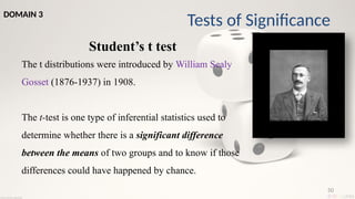
Student’s t test
Thet distributions were introduced by William Sealy
Gosset (1876-1937) in 1908.
The t-test is one type of inferential statistics used to
determine whether there is a significant difference
between the means of two groups and to know if those
differences could have happened by chance.
Tests of Significance
DOMAIN 3
46.
51
Student’s t test
Criteriafor applying t test
• The sample or samples must be randomly selected.
• The data must be quantitative.
• It can be used when sample size less than 30.
• when the data is normally distributed.
Tests of Significance
DOMAIN 3
47.
52
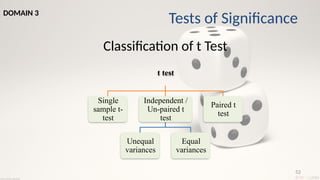
Classification of tTest
t test
Single
sample t-
test
Independent /
Un-paired t
test
Unequal
variances
Equal
variances
Paired t
test
Tests of Significance
DOMAIN 3
56
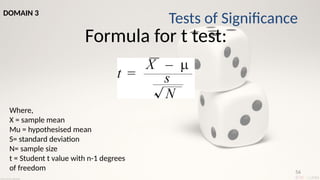
Formula for ttest:
Where,
X = sample mean
Mu = hypothesised mean
S= standard deviation
N= sample size
t = Student t value with n-1 degrees
of freedom
Tests of Significance
DOMAIN 3
52.
57
• Paired tTest (Paired Samples t Test / Dependent Samples t
Test)
( Before-and-after observations on the same subjects )
– The dependent variable must be continuous (interval/ratio).
– The observations are independent of one another.
– The dependent variable should be approximately normally
distributed.
– The dependent variable should not contain any outliers.
Tests of Significance
DOMAIN 3
53.
58
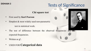
Chi square test
•First used by Karl Pearson
• Simplest & most widely used non-parametric
test in statistical work.
• The test of difference between the observed frequencies and the
expected frequencies.
• Written as χ2
.
• USED FOR Categorical data
Tests of Significance
DOMAIN 3
61
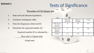
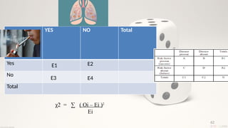
Procedure of Chi-Squaretest
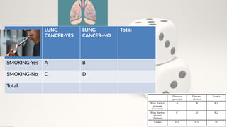
1. State null and alternate hypothesis.
2. Construct contingency table.
3. Note the frequencies observed (O)
4. Determine the expected number (E)
Expected number (E) is obtained by :
Row total x Column total
Grand total
Tests of Significance
DOMAIN 3
63
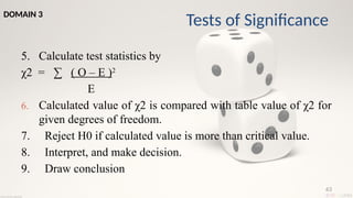
5. Calculate teststatistics by
χ2 = ∑ ( O – E )2
E
6. Calculated value of χ2 is compared with table value of χ2 for
given degrees of freedom.
7. Reject H0 if calculated value is more than critical value.
8. Interpret, and make decision.
9. Draw conclusion
Tests of Significance
DOMAIN 3
59.
64
3 unique functionsof χ2
test
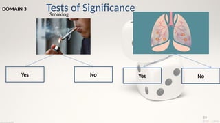
1. Test of association:
(smoking & cancer, treatment & outcome of disease, vaccination &
immunity)
2. Test of proportions:
(compare frequencies of diabetics & non-diabetics in groups
weighing 40-50kg, 50-60kg, 60-70kg & >70kg.)
3. The chi-square for goodness of fit:
(determine if actual numbers are similar to the expected/theoretical
numbers)
Tests of Significance
DOMAIN 3
60.
67
Multivariate Analysis
Introduction
• Multivariateanalysis consists of a collection of methods that can be used when several
measurements are made on each individual or object in one or more samples.
Application
• To equalize research groups
• To build causal models from observational studies
• To create clinical indices
Tests of Significance
DOMAIN 3
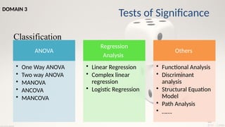
61.
68
Classification
ANOVA
• One WayANOVA
• Two way ANOVA
• MANOVA
• ANCOVA
• MANCOVA
Regression
Analysis
• Linear Regression
• Complex linear
regression
• Logistic Regression
Others
• Functional Analysis
• Discriminant
analysis
• Structural Equation
Model
• Path Analysis
• …….
Tests of Significance
DOMAIN 3
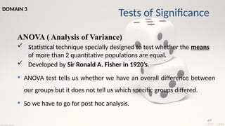
62.
69
ANOVA ( Analysisof Variance)
Statistical technique specially designed to test whether the means
of more than 2 quantitative populations are equal.
Developed by Sir Ronald A. Fisher in 1920’s.
ANOVA test tells us whether we have an overall difference between
our groups but it does not tell us which specific groups differed.
So we have to go for post hoc analysis.
Tests of Significance
DOMAIN 3
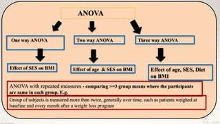
63.
70
ANOVA
One way ANOVAThree way ANOVA
Effect of SES on BMI
Two way ANOVA
Effect of age & SES on BMI Effect of age, SES, Diet
on BMI
ANOVA with repeated measures - comparing >=3 group means where the participants
are same in each group. E.g.
Group of subjects is measured more than twice, generally over time, such as patients weighed at
baseline and every month after a weight loss program
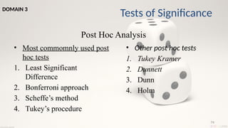
64.
Post Hoc Analysis
74
Testsof Significance
DOMAIN 3
• Most commomnly used post
hoc tests
1. Least Significant
Difference
2. Bonferroni approach
3. Scheffe’s method
4. Tukey’s procedure
• Other post hoc tests
1. Tukey Kramer
2. Dunnett
3. Dunn
4. Holm
65.
75
REGRESSION
• The RegressionAnalysis is a technique of studying the
dependence of one variable (called dependant variable), on one
or more variables (called independent variable), with a view to
estimate or predict the average value of the dependent variables in
terms of the known or fixed values of the independent variables.
Tests of Significance
DOMAIN 3
66.
76
Why Regression ??
•To find the significant relationships between dependent variable
and independent variable.
• To determine the strength of impact of multiple independent
variables on a dependent variable.
• To compare the effects of variables measured on different scales
Tests of Significance
DOMAIN 3
79
Types of Regression
•Linear regression : One outcome variable ( Continuous)
Predictor Variable(Continuous, Discrete)
i. Simple Linear regression
ii. Multiple Linear regression
• Logistic regression : One Outcome Variable - Dichotomous
Multiple Predictor variables – (
Continuous, discrete, interval, Ratio)
• Polynomial regression
• Stepwise regression
• Ridge regression
Tests of Significance
DOMAIN 3
70.
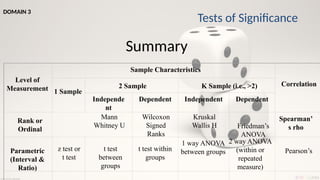
Summary
Level of
Measurement
Sample Characteristics
Correlation
1Sample
2 Sample K Sample (i.e., >2)
Independe
nt
Dependent Independent Dependent
Friedman’s
ANOVA
Parametric
(Interval &
Ratio)
z test or
t test
t test
between
groups
t test within
groups
1 way ANOVA
between groups
2 way ANOVA
(within or
repeated
measure)
Pearson’s
Rank or
Ordinal
Mann
Whitney U
Wilcoxon
Signed
Ranks
Kruskal
Wallis H
Spearman’
s rho
Tests of Significance
DOMAIN 3
82
Sample Size Estimation
Contents
•Introduction
• Rationale
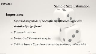
• Importance
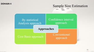
• Approaches
• Factors affecting the sample size
• Power of the study
• Methods of sample size estimation
• Conclusion
DOMAIN 4
73.
83
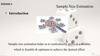
• Introduction
Sample sizeestimation helps us to meticulously arrive at a number,
which is feasible & optimum to achieve the desired effect.
Sample Size Estimation
DOMAIN 4
74.
84
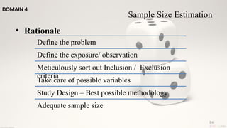
• Rationale
Sample SizeEstimation
Define the problem
Define the exposure/ observation
Meticulously sort out Inclusion / Exclusion
criteria
Take care of possible variables
Study Design – Best possible methodology
Adequate sample size
DOMAIN 4
87
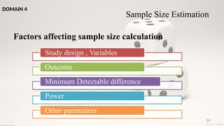
Factors affecting samplesize calculation
Study design , Variables
Outcome
Minimum Detectable difference
Power
Other paramaters
Sample Size Estimation
DOMAIN 4
78.
88
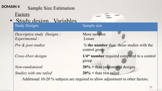
• Study design, Variables
Sample Size Estimation
Factors
Study Designs Sample size
Descriptive study Designs :
Experimental :
More samples
Lesser
Pre & post studies ½ the number than those studies with the
control group
Cross-Over designs 1/4th
number required compared to a control
group
Non-randomised 20% > than randomised designs
Studies with one tailed 20% < than two tailed
Additional 10-20 % subjects are required to allow adjustment to other factors.
DOMAIN 4
79.
89
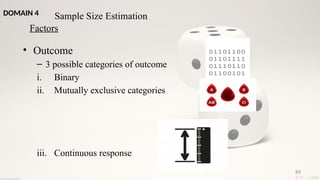
• Outcome
– 3possible categories of outcome
i. Binary
ii. Mutually exclusive categories
iii. Continuous response
Sample Size Estimation
Factors
DOMAIN 4
80.
90
• Minimum detectabledifference
Effect Size
Expected difference/
relationship between two
independent variables.
If available , it may be useful
to use the effect size found
from prior studies.
If not - Literature review,
logical assertion and
conjecture.
Sample Size Estimation
Factors
DOMAIN 4
81.
91
• Power ofthe study
– Statistical power means the probability of finding a
real effect (of the size that you think is clinically important)
– Ideally study should have high power
– High chances of detecting the difference if present
– The ideal power > 80%
Sample Size Estimation
Factors
DOMAIN 4
82.
92
Power of thestudy
In research – 2 objectives
1. Before data collection
2. After data analysis – when the data is non-significant
Sample Size Estimation
Factors
DOMAIN 4
83.
93
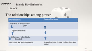
The relationships amongpower :
Sample Size Estimation
Factors
Parameters Power of the study
Variation in the Outcome
( SD)
Significance Level
Difference ( effect) to be
detected
One tailed vs. two tailed tests Power is greater in one –tailed than two
tailed.
DOMAIN 4
84.
94
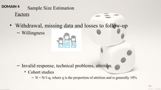
• Withdrawal, missingdata and losses to follow-up
– Willingness
– Invalid response, technical problems, attrition.
• Cohort studies
– N = N/1-q, where q is the proportion of attrition and is generally 10%
Sample Size Estimation
Factors
DOMAIN 4
85.
95
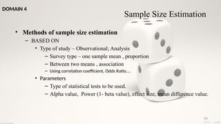
• Methods ofsample size estimation
– BASED ON
• Type of study – Observational; Analysis
– Survey type – one sample mean , proportion
– Between two means , association
– Using correlation coefficient, Odds Ratio….
• Parameters
– Type of statistical tests to be used.
– Alpha value, Power (1- beta value), effect size, mean difference value.
Sample Size Estimation
DOMAIN 4
86.
96
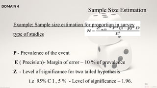
Example: Sample sizeestimation for proportion in survey
type of studies
P - Prevalence of the event
E ( Precision)- Margin of error – 10 % of prevalence
Z - Level of significance for two tailed hypothesis
i.e 95% C I , 5 % - Level of significance – 1.96.
Sample Size Estimation
DOMAIN 4
87.
97
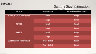
FACTOR MAGNITUDE REQUIREDSAMPLE SIZE
P VALUE OR ALPHA- LEVEL Small Large
Large Small
POWER Small Small
Large Large
EFFECT Small Large
Large Small
ALTERNATIVE HYPOTHESIS One - tailed Small
Two – tailed Large
Sample Size Estimation
DOMAIN 4
88.
98
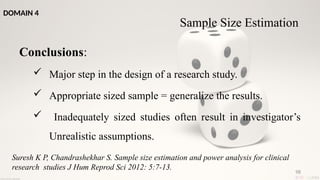
Conclusions:
Major stepin the design of a research study.
Appropriate sized sample = generalize the results.
Inadequately sized studies often result in investigator’s
Unrealistic assumptions.
Suresh K P, Chandrashekhar S. Sample size estimation and power analysis for clinical
research studies J Hum Reprod Sci 2012: 5:7-13.
DOMAIN 4
Sample Size Estimation
89.
99
• Other Domains- Short Notes
– Agreement & Diagnostic Tests
– Vital Statistics
– Bimodality
– Errors
– Odds Ratio
– Variables in Research
90.
100
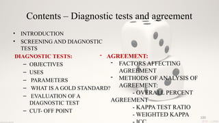
Contents – Diagnostictests and agreement
• INTRODUCTION
• SCREENING AND DIAGNOSTIC
TESTS
DIAGNOSTIC TESTS:
– OBJECTIVES
– USES
– PARAMETERS
– WHAT IS A GOLD STANDARD?
– EVALUATION OF A
DIAGNOSTIC TEST
– CUT- OFF POINT
- AGREEMENT:
- FACTORS AFFECTING
AGREEMENT
- METHODS OF ANALYSIS OF
AGREEMENT:
- OVERALL PERCENT
AGREEMENT
- KAPPA TEST RATIO
- WEIGHTED KAPPA
91.
101
References
1. Methods inbiostatistics for medical students and research
workers by BK Mahajan, 9th
edition.
2. Biostatistics for oral health care by Jay S. Kim, Ronald J. Dailey
3. Research methodology methods and techniques by C.R. Kothari,
4th
edition.
4. Introductory statistics by Prem S. Mann, 7th
edition.
5. Medical Statistics at a Glance by Aviva Petrie, 3rd
edition.
92.
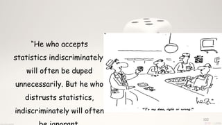
102
“He who accepts
statisticsindiscriminately,
will often be duped
unnecessarily. But he who
distrusts statistics,
indiscriminately will often
#4 Health statistics: In public health or community health
Medical statistics: In medicine related to the study of disease, efficacy, effectiveness of drug , efficiency of the prcedure etc
Vital statistics: In demography pertaining to vital events of births, marriages and deaths
These terms are overlapping and not exclusive of each other.
#5 1: Association of dental caries in low ses and high ses population
2. Efficacy of ART, Pit and fissures
3. Vaccine coverage, rate of addnission
4.
#6 To find what is normal or healthy in a population and to find limits of normality in variables
To find the correlation between 2 variables . Eg: Height and weight
To find relative potency of a new drug with respect to a standard drug
#7 2. TO find if a sign or symptom is charateristic of the disease under study or not.
Epidemiological studies: Studies relating sugar intake frequency and dental caries, fl and dental caries.
#8 1. Samples used in statistical tests that do not represent the population adequately can give reliable results but with little relevance to the population that it came from.
2. The qualitative phenomena like subjective phenomena, feelings, ratins , can not be analysed directly by statistical technique. However, they can be analysed once they are converted to some quantitative scores on suitable scales of measurement.
3. Statistics deals with aggregate of facts and does not give specific recognition to the individuals items of a series. Individual items taken separately does not constitute statistical data and meaningless for statistical enquiry. Statistical conclusions are not universally true. They are true on an average.
4. Unlike physical sciences, the statistical laws are only approximation and not exact. Statistics gives conclusion or decision in terms of probability not in terms of certainty.
5. The use of statistical tools by inexperienced untrained persons might lead to very fallacious conclusion.
#9 Descriptive statistics consists of methods for organizing, displaying, and describing data by using tables, graphs, and summary measures.
Inferential statistics consists of methods that use sample results to help make decisions or predictions about a population.
Primarily performed in two ways: Estimation and Testing of hypothesis
#10 Discrete : This type of data can’t be measured but it can be counted
Continuous Data: represents measurements and therefore their values can’t be counted but they can be measured.
It is defined as the data that is not precisely measurable by a scale, device, instrument or technique.
It describes the ‘quality’, ‘subjective’ or ‘non-numeric aspect’ of some characteristic.
#11 Nominal : data is expressed in categories, like blood groups, race, ..
Ordinal scale : Data is put into order, grade.
#15 Bar diagram
A bar diagram is a tool for comparing categories of mutually exclusive discrete data.
The different categories are indicated on one axis, the frequency of data in each category is indicated on the other axis, and the lengths of the bars compare the categories.
Pie chart
A pie chart is a pictorial representation of the proportional divisions of a sample or population, Degrees of angle denote frequency and area of sector
Angle = class frequency/total observation x 360
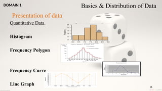
#16 Histogram : Depict quantitative data of continuous type
Frequency polygon:
Represents frequency distributions
Comparative analysis
Area diagram developed over a histogram
Point marked over mid point of class interval
Frequency curve: When the number of observations is very large and group interval is reduced, the frequency polygon tends to lose its angular appearance, giving place to a smooth curve known as frequency curve.
Line diagram : Simplest mean to represent data
Useful in representing trends over time
X –axis represent time
Y –axis , value of any variable under study
#19 The class or group interval between the groups should not be too broad or too narrow.
The class interval should be same throughout.
The classes must be mutually exclusive.
Contingency Table
Two-way table presenting relationship between 2 nominal or categorical variables
#22 The most common measure of central tendency
Unique for any quantitative data set
Balance point of a distribution
Disadvantages
Affected by extreme values (outliers)
Susceptible to the influence of outliers
Cannot be used for skewed data
Not ideal for qualitative data
#23 Sensitive to the sample size
Widely used for highly skewed distributions
Appropriate for ordinal variables
#24 Advantages
Only measure appropriate for nominal data.
Appropriate than mean or median for quantitative variables that are inherently discrete.
Simple to calculate.
Unaffected by extremely large or small values.
#25 It is the positive square root of the average of squares of deviations of the observations from the mean. This is also called root mean squared deviation (σ) .
#28 Normal distribution or Gaussian distribution is a continuous probability distribution of a large random sample.
The curve is continuous i.e, there are no gaps or holes.
#29 The shape of the normal distribution or curve tells the probability of occurrence by chance or how often an observation, measured in terms of mean and standard deviation can occur normally in a population.
#30 The left tail is longer; the mass of the distribution is concentrated on the right of the figure. The distribution is said to be left-skewed, left-tailed, or skewed to the left.A left-skewed distribution usually appears as a right-leaning curve.
The right tail is longer; the mass of the distribution is concentrated on the left of the figure. The distribution is said to be right-skewed, right-tailed, or skewed to the right.A right-skewed distribution usually appears as a left-leaning curve
#31 A distribution with positive excess kurtosis is called leptokurtic, In terms of shape, a leptokurtic distribution has fatter tails. Such distributions are sometimes termed super-Gaussian
A distribution with negative excess kurtosis is called platykurtic, or platykurtotic. "Platy-" means "broad". In terms of shape, a platykurtic distribution has thinner tails. Such distributions are sometimes termed sub-Gaussian.
#36 Errors can be during 1. Sampling 2. Research Process 3. During Analysis/ Statistics
The probability of committing a type I error is called α.“level of statistical significance”.
Type I error is usually fixed in advance by choice of the level of significance employed in the test.
#39 Step 3: It is important to note that we want to set α before the experiment (a-priori) because the Type I error is the more ‘grievous’ error to make. The typical value of α is 0.05, establishing a 95% confidence level.
Step 6: a threshold (critical) value of F is established. This F value can be obtained from statistical tables, and is referred to as Fcritical or Fα.
#41 Apart from these : Functional Analysis, Factor Analysis, ROC Curve, Agreement and Diagnostc Tests….
#50 writing under the pseudonym “Student” and hence referred to as the Student’s t test.
#52 three main types of t-test:
An Independent Samples t-test compares the means for two groups.
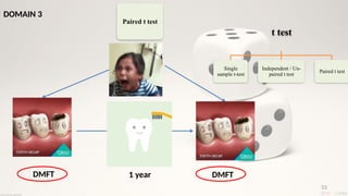
A Paired sample t-test compares means from the same group at different times (say, one year apart).
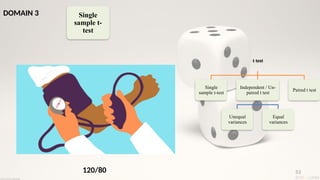
A One sample t-test tests the mean of a single group against a known mean.
#53 three main types of t-test:
An Independent Samples t-test compares the means for two groups.
A Paired sample t-test compares means from the same group at different times (say, one year apart).
A One sample t-test tests the mean of a single group against a known mean.
#54 three main types of t-test:
An Independent Samples t-test compares the means for two groups.
A Paired sample t-test compares means from the same group at different times (say, one year apart).
A One sample t-test tests the mean of a single group against a known mean.
#55 three main types of t-test:
An Independent Samples t-test compares the means for two groups.
A Paired sample t-test compares means from the same group at different times (say, one year apart).
A One sample t-test tests the mean of a single group against a known mean.
#57 Examples:
• Before-and-after observations on the same subjects (e.g. students’ diagnostic test results before and after a particular module or course).
• A comparison of two different methods of measurement or two different treatments where the measurements/treatments are applied to the same subjects
#58 X is the Greek letter “chi” pronounced “ki”.
All we can really look at are frequencies of occurrence.
If you have categorical data and you are wanting to see if the distributions are by chance or not.
#59 X is the Greek letter “chi” pronounced “ki”.
All we can really look at are frequencies of occurrence.
If you have categorical data and you are wanting to see if the distributions are by chance or not.
#61 O - in each class of one event, row-wise and the number in each group of the other event, column-wise.
E - in each group of the sample or the cell of table on the assumption of null hypothesis.
Eg….. put
#65 Fisher’s exact test
number of cases is <20 or
More than 25% of the cells have expected frequencies <5.
The Cochran-Mantel- Haenszel test : When the data is effected by confounding variable or 3rd variable.
McNemar’s test
Two related samples
There are repeated measurements and
In a matched analysis (for dichotomous variables)
#68 Multivariate analysis consists of a collection of methods that can be used when several measurements are made on each individual or object in one or more samples.
ANOVA is an extension of the 2 sample t test to 3 or more samples.
#75 FatherofRegressionAnalysis- Carl F. Gauss (1777-1855).
The term “Regression” was first used in 1877 by Francis Galton.
Regression analysis is a form of predictive modelling technique which investigates the relationship between a dependent (target) and independent variable (s) (predictor).
#83 As it is practically impossible to involve all the people into the study , we need to carefully plan the size, No. of the samples in order to achieve our objectives.
#89 The larger sammple size is required to assess the categotical variables compared to continuous outcome vairable
#91 Probability of refusing null hypothesis if alternative hypotheis is true.
Confidence interval indicate the the likely range of values for the true effect in the population/
P value determines how likely it is that the observed effect in the sample is due to chance.
#92 1. Based on the information from previous studies
2. In this case statistical power is calculated to verify whether the non-sig result is due to lack of relationship btw the groups or due to lack of statistical power
#93 Significance level = probability of a type I error = probability of finding an effect when there really isn't one. This is also known as alpha or α .
Probability of type II error = probability of failing to find an effect when there really is one. This is also known as beta or β.
Power = 1 – probability of type II error = probability of finding an effect when there really is one. This is also known as 1 – beta.


 Most read
 Most read
 Most read