Informed Search Strategies in Artificial Intelligence: Heuristics, Algorithms, and Applications
Explore informed search strategies in AI including heuristic functions, Greedy Best-First Search, A* algorithm, admissible and consistent heuristics, with practical examples and problem-solving techniques.
Informed Search Strategies in Artificial Intelligence: Heuristics, Algorithms, and Applications
1.
PCIT402 : ArtificialIntelligence
Sanjivani Rural Education Society’s
Sanjivani College of Engineering, Kopargaon-423603
(An Autonomous Institute Affiliated to Savitribai Phule Pune University, Pune)
NAAC ‘A’ Grade Accredited, ISO 9001:2015 Certified
Department of Information Technology
(UG Course: NBA Accredited)
Mr. R. N. Kankrale
Assistant Professor
2.
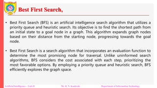
Unit-III INFORMED SEARCHSTRATEGIES
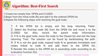
Artificial Intelligence – Overview Mr. R. N. Kankrale Department of Information Technology
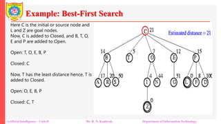
State-space representation and problem formulation
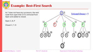
Uninformed search: BFS, DFS, Uniform Cost Search, Iterative Deepening Search
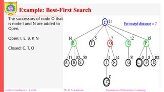
Informed search: Greedy Best-First Search, A* Search, AO* Search (overview)
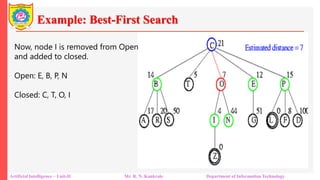
Heuristic functions, admissibility, and consistency
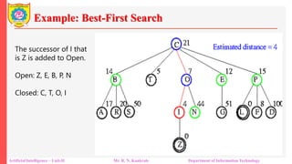
Local search: Hill Climbing, Simulated Annealing, Genetic Algorithms (overview)
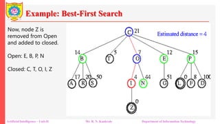
Game playing: Minimax Search and Alpha-Beta Pruning
Constraint Satisfaction Problems (CSP): N-Queens, Map Coloring
Illustrative examples: Water Jug Problem,8-Puzzle, Route Finding, Vacuum Cleaner World, Tic-Tac-Toe
3.
Informed Search(Heuristic Search)
ArtificialIntelligence – Unit-II Mr. R. N. Kankrale Department of Information Technology
INFORMED (HEURISTIC) SEARCH STRATEGIES
• Heuristic search strategies are like smart search methods that use special
knowledge or hints to find solutions more efficiently. It's similar to when we use
our intuition or common sense to solve a problem
4.
Informed Search(Heuristic Search)
ArtificialIntelligence – Unit-II Mr. R. N. Kankrale Department of Information Technology
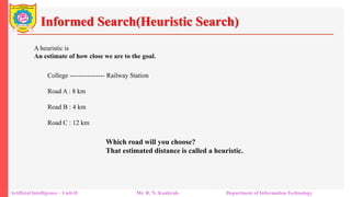
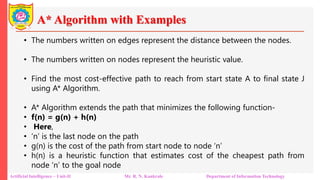
A heuristic is
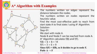
An estimate of how close we are to the goal.
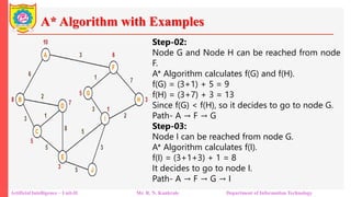
College ---------------- Railway Station
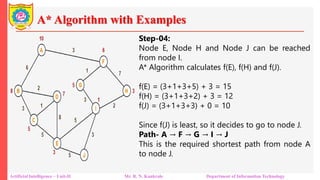
Road A : 8 km
Road B : 4 km
Road C : 12 km
Which road will you choose?
That estimated distance is called a heuristic.
5.
Informed Search(Heuristic Search)
ArtificialIntelligence – Unit-II Mr. R. N. Kankrale Department of Information Technology
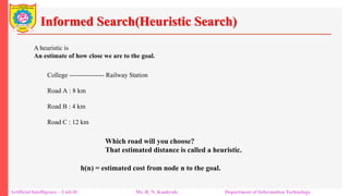
A heuristic is
An estimate of how close we are to the goal.
College ---------------- Railway Station
Road A : 8 km
Road B : 4 km
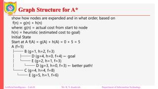
Road C : 12 km
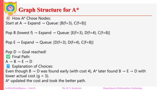
Which road will you choose?
That estimated distance is called a heuristic.
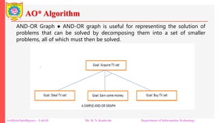
h(n) = estimated cost from node n to the goal.
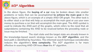
6.
Greedy Best-First Search
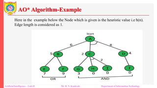
ArtificialIntelligence – Unit-II Mr. R. N. Kankrale Department of Information Technology
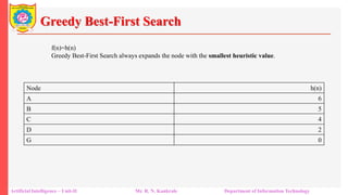
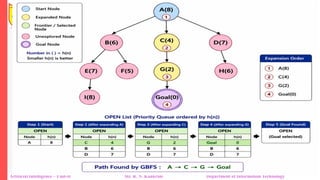
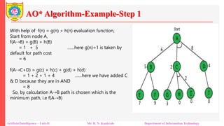
f(n)=h(n)
Greedy Best-First Search always expands the node with the smallest heuristic value.
Node h(n)
A 6
B 5
C 4
D 2
G 0
7.
Admissible Heuristic
Artificial Intelligence– Unit-II Mr. R. N. Kankrale Department of Information Technology
Suppose Google Maps says your college is 8 km away from the railway station.
Can the actual shortest road be only 6 km?
8.
Admissible Heuristic
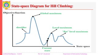
Artificial Intelligence– Unit-II Mr. R. N. Kankrale Department of Information Technology
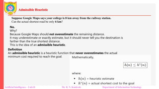
Suppose Google Maps says your college is 8 km away from the railway station.
Can the actual shortest road be only 6 km?
No.
Why?
Because Google Maps should not overestimate the remaining distance.
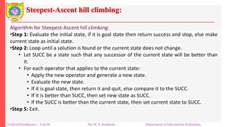
It may underestimate or exactly estimate, but it should never tell you the destination is
farther than the true shortest distance.
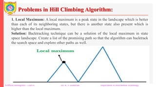
This is the idea of an admissible heuristic.
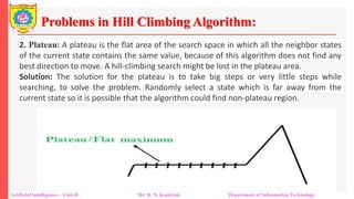
Definition
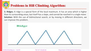
An admissible heuristic is a heuristic function that never overestimates the actual
minimum cost required to reach the goal.
9.
Admissible Heuristic
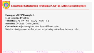
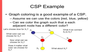
Artificial Intelligence– Unit-II Mr. R. N. Kankrale Department of Information Technology
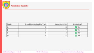
Node Actual Cost to Goal (h^*(n)) Heuristic (h(n)) Admissible?
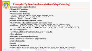
A 10 8 Yes
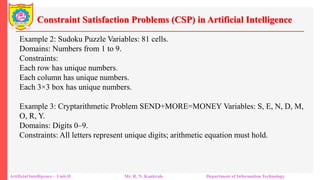
B 7 7 Yes
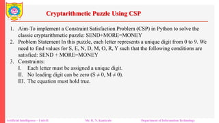
C 5 3 Yes
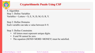
D 4 4 Yes
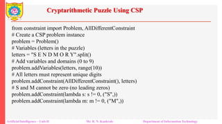
10.
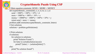
Greedy Best-First Search-Algorithm
ArtificialIntelligence – Unit-II Mr. R. N. Kankrale Department of Information Technology
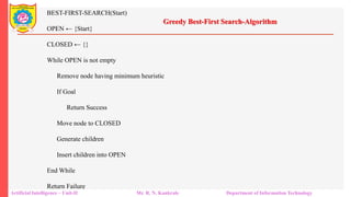
BEST-FIRST-SEARCH(Start)
OPEN ← {Start}
CLOSED ← {}
While OPEN is not empty
Remove node having minimum heuristic
If Goal
Return Success
Move node to CLOSED
Generate children
Insert children into OPEN
End While
Return Failure
11.
Greedy Best-First Search
ArtificialIntelligence – Unit-II Mr. R. N. Kankrale Department of Information Technology
f(n)=h(n)
Greedy Best-First Search always expands the node with the smallest heuristic value.
12.
Greedy Best-First Search
ArtificialIntelligence – Unit-II Mr. R. N. Kankrale Department of Information Technology
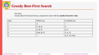
f(n)=h(n)
Greedy Best-First Search always expands the node with the smallest heuristic value.
Step OPEN List CLOSED List
1 A —
2 C, B, D A
3 G, B, D A, C
4 Goal, B, D A, C, G
5 — A, C, G, Goal
13.
Informed Search(Heuristic Search)
ArtificialIntelligence – Unit-II Mr. R. N. Kankrale Department of Information Technology
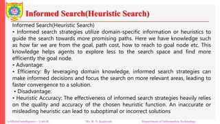
Informed Search(Heuristic Search)
• Informed search strategies utilize domain-specific information or heuristics to
guide the search towards more promising paths. Here we have knowledge such
as how far we are from the goal, path cost, how to reach to goal node etc. This
knowledge helps agents to explore less to the search space and find more
efficiently the goal node.
• Advantage:
• Efficiency: By leveraging domain knowledge, informed search strategies can
make informed decisions and focus the search on more relevant areas, leading to
faster convergence to a solution.
• Disadvantage:
• Heuristic Accuracy: The effectiveness of informed search strategies heavily relies
on the quality and accuracy of the chosen heuristic function. An inaccurate or
misleading heuristic can lead to suboptimal or incorrect solutions
14.
Best First Search,
ArtificialIntelligence – Unit-II Mr. R. N. Kankrale Department of Information Technology
• Best First Search (BFS) is an artificial intelligence search algorithm that utilizes a
priority queue and heuristic search. Its objective is to find the shortest path from
an initial state to a goal node in a graph. This algorithm expands graph nodes
based on their distance from the starting node, progressing towards the goal
node.
• Best First Search is a search algorithm that incorporates an evaluation function to
determine the most promising node for traversal. Unlike uninformed search
algorithms, BFS considers the cost associated with each step, prioritizing the
most favorable options. By employing a priority queue and heuristic search, BFS
efficiently explores the graph space.
15.
Algorithm: Best-First Search
ArtificialIntelligence – Unit-II Mr. R. N. Kankrale Department of Information Technology
1.Create two empty lists: OPEN and CLOSED.
2.Begin from the initial node (N) and add it to the ordered OPEN list.
3.Repeat the following steps until reaching the goal node:
1. If the OPEN list is empty, exit the loop, returning ‘False’.
2. Select the first/top node (N) from the OPEN list and move it to the
CLOSED list. Also, record the parent node information.
3. If N is the goal node, move the node to the Closed list and exit the loop
returning ‘True’. The solution can be found by backtracking the path.
4. If N is not the goal node, expand node N to generate immediate next
nodes linked to node N and add them to the OPEN list.
5 Reorder the nodes in the OPEN list in ascending order according to an
evaluation function f(n).
16.
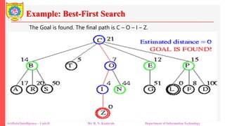
Example: Best-First Search
ArtificialIntelligence – Unit-II Mr. R. N. Kankrale Department of Information Technology
Here C is the initial or source node and
L and Z are goal nodes.
Now, C is added to Closed, and B, T, O,
E and P are added to Open.
Open: T, O, E, B, P
Closed: C
Now, T has the least distance hence, T is
added to Closed.
Open: O, E, B, P
Closed: C, T
17.
Example: Best-First Search
ArtificialIntelligence – Unit-II Mr. R. N. Kankrale Department of Information Technology
As T does not have any successors, the next
node from open that is O is removed from
Open and added to closed.
Open: E, B, P
Closed: C, T, O
18.
Example: Best-First Search
ArtificialIntelligence – Unit-II Mr. R. N. Kankrale Department of Information Technology
The successors of node O that
is node I and N are added to
Open.
Open: I, E, B, P, N
Closed: C, T, O
19.
Example: Best-First Search
ArtificialIntelligence – Unit-II Mr. R. N. Kankrale Department of Information Technology
Now, node I is removed from Open
and added to closed.
Open: E, B, P, N
Closed: C, T, O, I
20.
Example: Best-First Search
ArtificialIntelligence – Unit-II Mr. R. N. Kankrale Department of Information Technology
The successor of I that
is Z is added to Open.
Open: Z, E, B, P, N
Closed: C, T, O, I
21.
Example: Best-First Search
ArtificialIntelligence – Unit-II Mr. R. N. Kankrale Department of Information Technology
Now, node Z is
removed from Open
and added to closed.
Open: E, B, P, N
Closed: C, T, O, I, Z
22.
Example: Best-First Search
ArtificialIntelligence – Unit-II Mr. R. N. Kankrale Department of Information Technology
The Goal is found. The final path is C – O – I – Z.
23.
Consistent Heuristic
Artificial Intelligence– Unit-II Mr. R. N. Kankrale Department of Information Technology
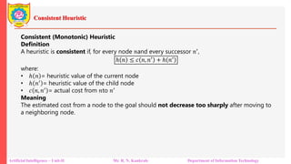
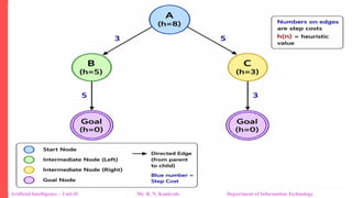
Consistent (Monotonic) Heuristic
Definition
A heuristic is consistent if, for every node 𝑛and every successor 𝑛′,
ℎ 𝑛 ≤ 𝑐 𝑛 𝑛′ + ℎ 𝑛′
where:
• ℎ 𝑛 = heuristic value of the current node
• ℎ 𝑛′ = heuristic value of the child node
• 𝑐 𝑛 𝑛′ = actual cost from 𝑛to 𝑛′
Meaning
The estimated cost from a node to the goal should not decrease too sharply after moving to
a neighboring node.
A* Algorithm
Artificial Intelligence– Unit-II Mr. R. N. Kankrale Department of Information Technology
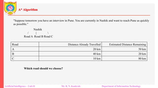
"Suppose tomorrow you have an interview in Pune. You are currently in Nashik and want to reach Pune as quickly
as possible."
Nashik
/ |
Road A Road B Road C
Road Distance Already Travelled Estimated Distance Remaining
A 20 km 50 km
B 40 km 20 km
C 10 km 80 km
Which road should we choose?
26.
A* Algorithm
Artificial Intelligence– Unit-II Mr. R. N. Kankrale Department of Information Technology
"Wait... haven't we already travelled 40 km on Road B? Shouldn't that matter?"
27.
A* Algorithm
Artificial Intelligence– Unit-II Mr. R. N. Kankrale Department of Information Technology
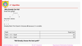
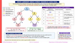
Why Greedy Can Fail
Draw this graph.
Start
/
A B
Heuristic values:
A = 2
B = 5
Greedy Best-First Search chooses A because 2 is smaller.
Path Total Cost
Start → A → Goal 25
Start → B → Goal 10
"Did Greedy choose the best path?"
28.
A* Algorithm
Artificial Intelligence– Unit-II Mr. R. N. Kankrale Department of Information Technology
Greedy only looked at the remaining distance.
It ignored the distance already travelled.
"A smart driver should consider two things:
1. How far have I already travelled?
2. How far is left?"
This is exactly what A* does.
29.
A* Algorithm
Artificial Intelligence– Unit-II Mr. R. N. Kankrale Department of Information Technology
Greedy only looked at the remaining distance.
It ignored the distance already travelled.
"A smart driver should consider two things:
1. How far have I already travelled?
2. How far is left?"
This is exactly what A* does.
30.
A* Algorithm
Artificial Intelligence– Unit-II Mr. R. N. Kankrale Department of Information Technology
"Wait... haven't we already travelled 40 km on Road B? Shouldn't that matter?"
31.
A* Algorithm
Artificial Intelligence– Unit-II Mr. R. N. Kankrale Department of Information Technology
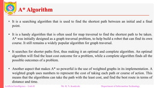
• It is a searching algorithm that is used to find the shortest path between an initial and a final
point.
• It is a handy algorithm that is often used for map traversal to find the shortest path to be taken.
A* was initially designed as a graph traversal problem, to help build a robot that can find its own
course. It still remains a widely popular algorithm for graph traversal.
• It searches for shorter paths first, thus making it an optimal and complete algorithm. An optimal
algorithm will find the least cost outcome for a problem, while a complete algorithm finds all the
possible outcomes of a problem.
• Another aspect that makes A* so powerful is the use of weighted graphs in its implementation. A
weighted graph uses numbers to represent the cost of taking each path or course of action. This
means that the algorithms can take the path with the least cost, and find the best route in terms of
distance and time.
32.
A* Algorithm
Artificial Intelligence– Unit-II Mr. R. N. Kankrale Department of Information Technology
Applications of A* Algorithm
The A* algorithm is widely used in various domains for pathfinding and optimization
problems. It has applications in robotics, video games, route planning, logistics, and
artificial intelligence. In robotics, A* helps robots navigate obstacles and find optimal
paths. In video games, it enables NPCs to navigate game environments intelligently.
Route planning applications use A* to find the shortest or fastest routes between
locations. Logistics industries utilize A* for vehicle routing and scheduling. A* is also
employed in AI systems, such as natural language processing and machine learning, to
optimize decision-making processes. Its versatility and efficiency make it a valuable
algorithm in many real-world scenarios.
33.
A* Algorithm withExamples
Artificial Intelligence – Unit-II Mr. R. N. Kankrale Department of Information Technology
34.
A* Algorithm withExamples
Artificial Intelligence – Unit-II Mr. R. N. Kankrale Department of Information Technology
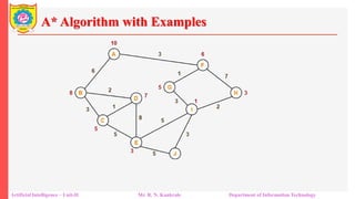
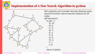
• The numbers written on edges represent the distance between the nodes.
• The numbers written on nodes represent the heuristic value.
• Find the most cost-effective path to reach from start state A to final state J
using A* Algorithm.
• A* Algorithm extends the path that minimizes the following function-
• f(n) = g(n) + h(n)
• Here,
• ‘n’ is the last node on the path
• g(n) is the cost of the path from start node to node ‘n’
• h(n) is a heuristic function that estimates cost of the cheapest path from
node ‘n’ to the goal node
35.
A* Algorithm withExamples
Artificial Intelligence – Unit-II Mr. R. N. Kankrale Department of Information Technology
The numbers written on edges represent the
distance between the nodes.
The numbers written on nodes represent the
heuristic value.
Find the most cost-effective path to reach from
start state A to final state J using A* Algorithm.
Solution-
Step-01:
We start with node A.
Node B and Node F can be reached from node A.
A* Algorithm calculates f(B) and f(F).
f(B) = 6 + 8 = 14
f(F) = 3 + 6 = 9
Since f(F) < f(B), so it decides to go to node F.
Path- A → F
36.
A* Algorithm withExamples
Artificial Intelligence – Unit-II Mr. R. N. Kankrale Department of Information Technology
Step-02:
Node G and Node H can be reached from node
F.
A* Algorithm calculates f(G) and f(H).
f(G) = (3+1) + 5 = 9
f(H) = (3+7) + 3 = 13
Since f(G) < f(H), so it decides to go to node G.
Path- A → F → G
Step-03:
Node I can be reached from node G.
A* Algorithm calculates f(I).
f(I) = (3+1+3) + 1 = 8
It decides to go to node I.
Path- A → F → G → I
37.
A* Algorithm withExamples
Artificial Intelligence – Unit-II Mr. R. N. Kankrale Department of Information Technology
Step-04:
Node E, Node H and Node J can be reached
from node I.
A* Algorithm calculates f(E), f(H) and f(J).
f(E) = (3+1+3+5) + 3 = 15
f(H) = (3+1+3+2) + 3 = 12
f(J) = (3+1+3+3) + 0 = 10
Since f(J) is least, so it decides to go to node J.
Path- A → F → G → I → J
This is the required shortest path from node A
to node J.
38.
PRACTICE PROBLEMS BASEDON A* ALGORITHM-
Artificial Intelligence – Unit-II Mr. R. N. Kankrale Department of Information Technology
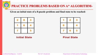
Given an initial state of a 8-puzzle problem and final state to be reached-
39.
PRACTICE PROBLEMS BASEDON A* ALGORITHM-
Artificial Intelligence – Unit-II Mr. R. N. Kankrale Department of Information Technology
Given an initial state of a 8-puzzle problem and final state to be reached-
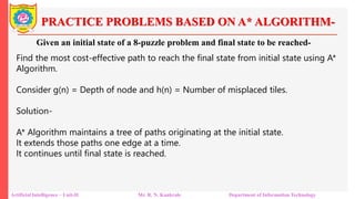
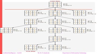
Find the most cost-effective path to reach the final state from initial state using A*
Algorithm.
Consider g(n) = Depth of node and h(n) = Number of misplaced tiles.
Solution-
A* Algorithm maintains a tree of paths originating at the initial state.
It extends those paths one edge at a time.
It continues until final state is reached.
A* Algorithm withExamples
Artificial Intelligence – Unit-II Mr. R. N. Kankrale Department of Information Technology
• Algorithm-
• The implementation of A* Algorithm involves maintaining two lists- OPEN
and CLOSED.
• OPEN contains those nodes that have been evaluated by the heuristic
function but have not been expanded into successors yet.
• CLOSED contains those nodes that have already been visited.
• The algorithm is as follows-
Step-01:
•Define a list OPEN.
•Initially, OPEN consists solely of a single node, the start node S.
42.
A* Algorithm withExamples
Artificial Intelligence – Unit-II Mr. R. N. Kankrale Department of Information Technology
Step-02:
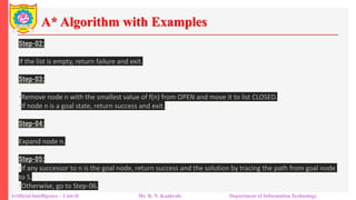
If the list is empty, return failure and exit.
Step-03:
•Remove node n with the smallest value of f(n) from OPEN and move it to list CLOSED.
•If node n is a goal state, return success and exit.
Step-04:
Expand node n.
Step-05:
•If any successor to n is the goal node, return success and the solution by tracing the path from goal node
to S.
•Otherwise, go to Step-06.
43.
A* Algorithm withExamples
Artificial Intelligence – Unit-II Mr. R. N. Kankrale Department of Information Technology
Step-06:
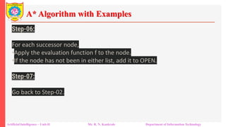
For each successor node,
•Apply the evaluation function f to the node.
•If the node has not been in either list, add it to OPEN.
Step-07:
Go back to Step-02.
44.
Implementation of AStar Search Algorithm in python
Artificial Intelligence – Unit-II Mr. R. N. Kankrale Department of Information Technology
#for simplicity we ll consider heuristic distances given
#and this function returns heuristic distance for all
nodes
def heuristic(n):
H_dist = {
'A’: 10,
'B': 6,
'C': 5,
'D': 7,
'E': 3,
'F': 6,
'G': 5,
'H': 3,
'I': 1,
'J': 0
}
return H_dist[n]
45.
Implementation of AStar Search Algorithm in python
Artificial Intelligence – Unit-II Mr. R. N. Kankrale Department of Information Technology
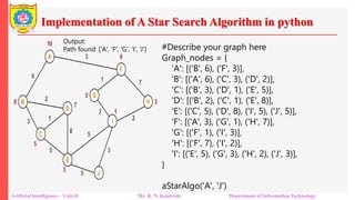
#Describe your graph here
Graph_nodes = {
'A': [('B', 6), ('F', 3)],
'B': [('A', 6), ('C', 3), ('D', 2)],
'C': [('B', 3), ('D', 1), ('E', 5)],
'D': [('B', 2), ('C', 1), ('E', 8)],
'E': [('C', 5), ('D', 8), ('I', 5), ('J', 5)],
'F': [('A', 3), ('G', 1), ('H', 7)],
'G': [('F', 1), ('I', 3)],
'H': [('F', 7), ('I', 2)],
'I': [('E', 5), ('G', 3), ('H', 2), ('J', 3)],
}
aStarAlgo('A', 'J')
Output:
Path found: ['A', 'F', 'G', 'I', ‘J’]
46.
Implementation of AStar Search Algorithm in python
Artificial Intelligence – Unit-II Mr. R. N. Kankrale Department of Information Technology
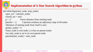
def aStarAlgo(start_node, stop_node):
open_set = set(start_node)
closed_set = set()
g = {} #store distance from starting node
parents = {} # parents contains an adjacency map of all nodes
#distance of starting node from itself is zero
g[start_node] = 0
#start_node is root node i.e it has no parent nodes
#so start_node is set to its own parent node
parents[start_node] = start_node
47.
Implementation of AStar Search Algorithm in python
Artificial Intelligence – Unit-II Mr. R. N. Kankrale Department of Information Technology
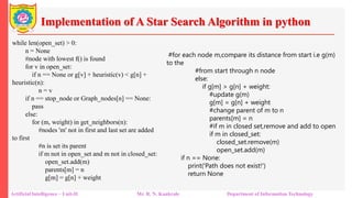
while len(open_set) > 0:
n = None
#node with lowest f() is found
for v in open_set:
if n == None or g[v] + heuristic(v) < g[n] +
heuristic(n):
n = v
if n == stop_node or Graph_nodes[n] == None:
pass
else:
for (m, weight) in get_neighbors(n):
#nodes 'm' not in first and last set are added
to first
#n is set its parent
if m not in open_set and m not in closed_set:
open_set.add(m)
parents[m] = n
g[m] = g[n] + weight
#for each node m,compare its distance from start i.e g(m)
to the
#from start through n node
else:
if g[m] > g[n] + weight:
#update g(m)
g[m] = g[n] + weight
#change parent of m to n
parents[m] = n
#if m in closed set,remove and add to open
if m in closed_set:
closed_set.remove(m)
open_set.add(m)
if n == None:
print('Path does not exist!')
return None
48.
Implementation of AStar Search Algorithm in python
Artificial Intelligence – Unit-II Mr. R. N. Kankrale Department of Information Technology
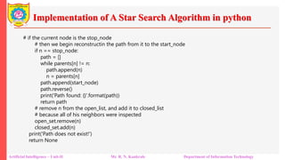
# if the current node is the stop_node
# then we begin reconstructin the path from it to the start_node
if n == stop_node:
path = []
while parents[n] != n:
path.append(n)
n = parents[n]
path.append(start_node)
path.reverse()
print('Path found: {}'.format(path))
return path
# remove n from the open_list, and add it to closed_list
# because all of his neighbors were inspected
open_set.remove(n)
closed_set.add(n)
print('Path does not exist!')
return None
49.
Implementation of AStar Search Algorithm in python
Artificial Intelligence – Unit-II Mr. R. N. Kankrale Department of Information Technology
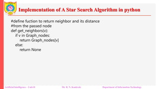
#define fuction to return neighbor and its distance
#from the passed node
def get_neighbors(v):
if v in Graph_nodes:
return Graph_nodes[v]
else:
return None
50.
Graph Structure forA*
Artificial Intelligence – Unit-II Mr. R. N. Kankrale Department of Information Technology
show how nodes are expanded and in what order, based on
f(n) = g(n) + h(n)
where: g(n) = actual cost from start to node
h(n) = heuristic (estimated cost to goal)
Initial State
Start at A f(A) = g(A) + h(A) = 0 + 5 = 5
A (f=5)
├── B (g=1, h=2, f=3)
│ ├── D (g=4, h=0, f=4) ← goal
│ └── E (g=2, h=1, f=3)
│ └── D (g=3, h=0, f=3) ← better path!
└── C (g=4, h=4, f=8)
└── E (g=5, h=1, f=6)
51.
Graph Structure forA*
Artificial Intelligence – Unit-II Mr. R. N. Kankrale Department of Information Technology
How A* Chose Nodes:
Start at A → Expand → Queue: [B(f=3), C(f=8)]
Pop B (lowest f) → Expand → Queue: [E(f=3), D(f=4), C(f=8)]
Pop E → Expand → Queue: [D(f=3), D(f=4), C(f=8)]
Pop D → Goal reached!
Final Path:
A → B → E → D
Explanation of Choices:
Even though B → D was found early (with cost 4), A* later found B → E → D with
lower actual cost (g = 3).
A* updated the cost and took the better path.
52.
AO* Algorithm -AO*Search (And-Or) Graph
Artificial Intelligence – Unit-II Mr. R. N. Kankrale Department of Information Technology
Introduction
● Its an informed search and works as best first search.
● AO* Algorithm is based on problem decomposition (Breakdown
problem into small pieces).
● Its an efficient method to explore a solution path.
● AO* is often used for the common pathfinding problem in applications
such as video games, but was originally designed as a general graph
traversal algorithm.
● It finds applications in diverse problems, including the problem of
parsing using stochastic grammars in NLP.
● Other cases include an Informational search with online learning.
● It is useful for searching game trees, problem solving etc.
53.
AO* Algorithm
Artificial Intelligence– Unit-II Mr. R. N. Kankrale Department of Information Technology
AND-OR Graph ● AND-OR graph is useful for representing the solution of
problems that can be solved by decomposing them into a set of smaller
problems, all of which must then be solved.
54.
AO* Algorithm
Artificial Intelligence– Unit-II Mr. R. N. Kankrale Department of Information Technology
In the above figure, the buying of a car may be broken down into smaller
problems or tasks that can be accomplished to achieve the main goal in the
above figure, which is an example of a simple AND-OR graph. The other task is
to either steal a car that will help us accomplish the main goal or use your own
money to purchase a car that will accomplish the main goal. The AND symbol is
used to indicate the AND part of the graphs, which refers to the need that all
subproblems containing the AND to be resolved before the preceding node or
issue may be finished.
The start state and the target state are already known in
the knowledge-based search strategy known as the AO* algorithm, and the
best path is identified by heuristics. The informed search technique considerably
reduces the algorithm’s time complexity. The AO* algorithm is far more
effective in searching AND-OR trees than the A* algorithm.
55.
AO* Algorithm
Artificial Intelligence– Unit-II Mr. R. N. Kankrale Department of Information Technology
AND-OR Graph
● Node in the graph will point both down to its successors and up to its parent
nodes.
● Each Node in the graph will also have a heuristic value associated with it.
f(n)=g(n)+h(n)
f(n): Cost function.
g(n): Actual cost or Edge value
h(n): Heuristic/ Estimated value of the nodes
56.
AO* Algorithm-Example
Artificial Intelligence– Unit-II Mr. R. N. Kankrale Department of Information Technology
Here in the example below the Node which is given is the heuristic value i.e h(n).
Edge length is considered as 1.
57.
AO* Algorithm-Example-Step 1
ArtificialIntelligence – Unit-II Mr. R. N. Kankrale Department of Information Technology
With help of f(n) = g(n) + h(n) evaluation function,
Start from node A,
f(A⇢B) = g(B) + h(B)
= 1 + 5 ……here g(n)=1 is taken by
default for path cost
= 6
f(A⇢C+D) = g(c) + h(c) + g(d) + h(d)
= 1 + 2 + 1 + 4 ……here we have added C
& D because they are in AND
= 8
So, by calculation A⇢B path is chosen which is the
minimum path, i.e f(A⇢B)
58.
AO* Algorithm-Example-Step 2
ArtificialIntelligence – Unit-II Mr. R. N. Kankrale Department of Information Technology
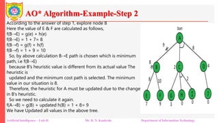
According to the answer of step 1, explore node B
Here the value of E & F are calculated as follows,
f(B⇢E) = g(e) + h(e)
f(B⇢E) = 1 + 7= 8
f(B⇢f) = g(f) + h(f)
f(B⇢f) = 1 + 9 = 10
So, by above calculation B⇢E path is chosen which is minimum
path, i.e f(B⇢E)
because B's heuristic value is different from its actual value The
heuristic is
updated and the minimum cost path is selected. The minimum
value in our situation is 8.
Therefore, the heuristic for A must be updated due to the change
in B's heuristic.
So we need to calculate it again.
f(A⇢B) = g(B) + updated h(B) = 1 + 8= 9
We have Updated all values in the above tree.
59.
AO* Algorithm-Example-Step 3
ArtificialIntelligence – Unit-II Mr. R. N. Kankrale Department of Information Technology
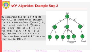
By comparing f(A⇢B) & f(A⇢C+D)
f(A⇢C+D) is shown to be smaller.
i.e 8 < 9 Now explore f(A⇢C+D) So,
the current node is C f(C⇢G) =
g(g) + h(g) f(C⇢G) = 1 + 3 = 4
f(C⇢H+I) = g(h) + h(h) + g(i) +
h(i) f(C⇢H+I) = 1 + 0 + 1 + 0
……here we have added H & I because
they are in AND = 2
60.
AO* Algorithm-Example-Step 3
ArtificialIntelligence – Unit-II Mr. R. N. Kankrale Department of Information Technology
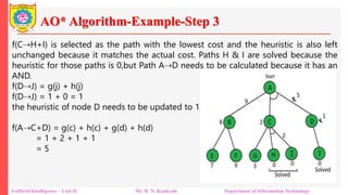
f(C⇢H+I) is selected as the path with the lowest cost and the heuristic is also left
unchanged because it matches the actual cost. Paths H & I are solved because the
heuristic for those paths is 0,but Path A⇢D needs to be calculated because it has an
AND.
f(D⇢J) = g(j) + h(j)
f(D⇢J) = 1 + 0 = 1
the heuristic of node D needs to be updated to 1.
f(A⇢C+D) = g(c) + h(c) + g(d) + h(d)
= 1 + 2 + 1 + 1
= 5
61.
Difference between theA* Algorithm and AO* algorithm
Artificial Intelligence – Unit-II Mr. R. N. Kankrale Department of Information Technology
•A* algorithm and AO* algorithm both works on the best first search.
•They are both informed search and works on given heuristics values.
•A* always gives the optimal solution but AO* doesn’t guarantee to give the optimal
solution.
•Once AO* got a solution doesn’t explore all possible paths but A* explores all paths.
•When compared to the A* algorithm, the AO* algorithm uses less memory.
•opposite to the A* algorithm, the AO* algorithm cannot go into an endless loop.
62.
Advantages and Disadvantagesof Best First Search
Artificial Intelligence – Unit-II Mr. R. N. Kankrale Department of Information Technology
Advantages
•Ability to switch between Breadth-First Search (BFS) and Depth-First Search (DFS),
gaining the advantages of both.
•More efficient compared to Depth-First Search.
Disadvantages
•Increased risk of getting stuck in a loop.
63.
Generate & Test
ArtificialIntelligence – Unit-II Mr. R. N. Kankrale Department of Information Technology
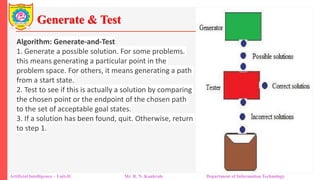
Algorithm: Generate-and-Test
1. Generate a possible solution. For some problems.
this means generating a particular point in the
problem space. For others, it means generating a path
from a start state.
2. Test to see if this is actually a solution by comparing
the chosen point or the endpoint of the chosen path
to the set of acceptable goal states.
3. If a solution has been found, quit. Otherwise, return
to step 1.
64.
Generate & Test
ArtificialIntelligence – Unit-II Mr. R. N. Kankrale Department of Information Technology
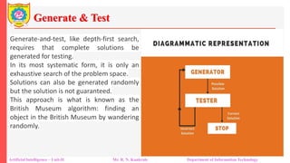
Generate-and-test, like depth-first search,
requires that complete solutions be
generated for testing.
In its most systematic form, it is only an
exhaustive search of the problem space.
Solutions can also be generated randomly
but the solution is not guaranteed.
This approach is what is known as the
British Museum algorithm: finding an
object in the British Museum by wandering
randomly.
65.
Generate & Test
ArtificialIntelligence – Unit-II Mr. R. N. Kankrale Department of Information Technology
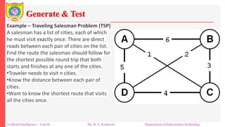
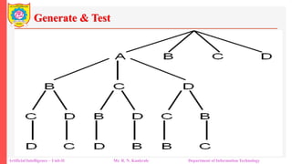
Example – Traveling Salesman Problem (TSP)
A salesman has a list of cities, each of which
he must visit exactly once. There are direct
roads between each pair of cities on the list.
Find the route the salesman should follow for
the shortest possible round trip that both
starts and finishes at any one of the cities.
•Traveler needs to visit n cities.
•Know the distance between each pair of
cities.
•Want to know the shortest route that visits
all the cities once.
66.
Generate & Test
ArtificialIntelligence – Unit-II Mr. R. N. Kankrale Department of Information Technology
67.
Generate & Test
ArtificialIntelligence – Unit-II Mr. R. N. Kankrale Department of Information Technology
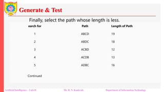
earch for Path Length of Path
1 ABCD 19
2 ABDC 18
3 ACBD 12
4 ACDB 13
5 ADBC 16
Continued
Finally, select the path whose length is less.
68.
Hill Climbing
Artificial Intelligence– Unit-II Mr. R. N. Kankrale Department of Information Technology
Hill climbing search algorithm is simply a loop that continuously moves in the
direction of increasing value. It stops when it reaches a “peak” where no neighbor has
higher value. This algorithm is considered to be one of the simplest procedures for
implementing heuristic search. The hill climbing comes from that idea if you are trying
to find the top of the hill and you go up direction from where ever you are. This
heuristic combines the advantages of both depth first and breadth first searches into a
single method.
69.
Hill Climbing,
Artificial Intelligence– Unit-II Mr. R. N. Kankrale Department of Information Technology
The name hill climbing is derived from simulating the situation of a person climbing the hill.
The person will try to move forward in the direction of at the top of the hill. His movement
stops when it reaches at the peak of hill and no peak has higher value of heuristic function
than this. Hill climbing uses knowledge about the local terrain, providing a very useful and
effective heuristic for eliminating much of the unproductive search space. It is a branch by a
local evaluation function.
The hill climbing is a variant of generate and test in which direction the search should
proceed. At each point in the search path, a successor node that appears to reach for
exploration.
70.
Features of HillClimbing:
Artificial Intelligence – Unit-II Mr. R. N. Kankrale Department of Information Technology
Features of Hill Climbing:
Following are some main features of Hill Climbing Algorithm:
•Generate and Test variant: Hill Climbing is the variant of Generate and Test method. The
Generate and Test method produce feedback which helps to decide which direction to move
in the search space.
•Greedy approach: Hill-climbing algorithm search moves in the direction which optimizes
the cost.
•No backtracking: It does not backtrack the search space, as it does not remember the
previous states.
71.
State-space Diagram forHill Climbing:
Artificial Intelligence – Unit-II Mr. R. N. Kankrale Department of Information Technology
72.
State-space Diagram forHill Climbing:
Artificial Intelligence – Unit-II Mr. R. N. Kankrale Department of Information Technology
The state-space landscape is a graphical representation of the hill-climbing algorithm
which is showing a graph between various states of algorithm and Objective function/Cost.
On Y-axis we have taken the function which can be an objective function or cost function,
and state-space on the x-axis. If the function on Y-axis is cost then, the goal of search is to
find the global minimum and local minimum. If the function of Y-axis is Objective
function, then the goal of the search is to find the global maximum and local maximum.
73.
Different regions inthe state space landscape:
Artificial Intelligence – Unit-II Mr. R. N. Kankrale Department of Information Technology
Local Maximum: Local maximum is a state which is better than its neighbor states,
but there is also another state which is higher than it.
Global Maximum: Global maximum is the best possible state of state space landscape.
It has the highest value of objective function.
Current state: It is a state in a landscape diagram where an agent is currently present.
Flat local maximum: It is a flat space in the landscape where all the neighbor states of
current states have the same value.
Shoulder: It is a plateau region which has an uphill edge.
74.
Types of HillClimbing Algorithm:
Artificial Intelligence – Unit-II Mr. R. N. Kankrale Department of Information Technology
•Simple hill Climbing:
•Steepest-Ascent hill-climbing:
•Stochastic hill Climbing:
75.
Simple hill Climbing:
ArtificialIntelligence – Unit-II Mr. R. N. Kankrale Department of Information Technology
Simple hill climbing is the simplest way to implement a hill climbing algorithm. It only
evaluates the neighbor node state at a time and selects the first one which optimizes
current cost and set it as a current state. It only checks it's one successor state, and if it
finds better than the current state, then move else be in the same state. This algorithm
has the following features:
•Less time consuming
•Less optimal solution and the solution is not guaranteed
76.
Simple hill Climbing:
ArtificialIntelligence – Unit-II Mr. R. N. Kankrale Department of Information Technology
Algorithm for Simple Hill Climbing:
•Step 1: Evaluate the initial state, if it is goal state then return success and Stop.
•Step 2: Loop Until a solution is found or there is no new operator left to apply.
•Step 3: Select and apply an operator to the current state.
•Step 4: Check new state:
• If it is goal state, then return success and quit.
• Else if it is better than the current state then assign new state as a current state.
• Else if not better than the current state, then return to step2.
•Step 5: Exit.
77.
Steepest-Ascent hill climbing:
ArtificialIntelligence – Unit-II Mr. R. N. Kankrale Department of Information Technology
The steepest-Ascent algorithm is a variation of simple hill climbing algorithm.
This algorithm examines all the neighboring nodes of the current state and
selects one neighbor node which is closest to the goal state. This algorithm
consumes more time as it searches for multiple neighbors
78.
Steepest-Ascent hill climbing:
ArtificialIntelligence – Unit-II Mr. R. N. Kankrale Department of Information Technology
Algorithm for Steepest-Ascent hill climbing:
•Step 1: Evaluate the initial state, if it is goal state then return success and stop, else make
current state as initial state.
•Step 2: Loop until a solution is found or the current state does not change.
• Let SUCC be a state such that any successor of the current state will be better than
it.
• For each operator that applies to the current state:
• Apply the new operator and generate a new state.
• Evaluate the new state.
• If it is goal state, then return it and quit, else compare it to the SUCC.
• If it is better than SUCC, then set new state as SUCC.
• If the SUCC is better than the current state, then set current state to SUCC.
•Step 5: Exit.
79.
Stochastic hill climbing:
ArtificialIntelligence – Unit-II Mr. R. N. Kankrale Department of Information Technology
Stochastic hill climbing:
Stochastic hill climbing does not examine for all its neighbor before moving. Rather,
this search algorithm selects one neighbor node at random and decides whether to
choose it as a current state or examine another state.
80.
Problems in HillClimbing Algorithm:
Artificial Intelligence – Unit-II Mr. R. N. Kankrale Department of Information Technology
1. Local Maximum: A local maximum is a peak state in the landscape which is better
than each of its neighboring states, but there is another state also present which is
higher than the local maximum.
Solution: Backtracking technique can be a solution of the local maximum in state
space landscape. Create a list of the promising path so that the algorithm can backtrack
the search space and explore other paths as well.
81.
Problems in HillClimbing Algorithm:
Artificial Intelligence – Unit-II Mr. R. N. Kankrale Department of Information Technology
2. Plateau: A plateau is the flat area of the search space in which all the neighbor states
of the current state contains the same value, because of this algorithm does not find any
best direction to move. A hill-climbing search might be lost in the plateau area.
Solution: The solution for the plateau is to take big steps or very little steps while
searching, to solve the problem. Randomly select a state which is far away from the
current state so it is possible that the algorithm could find non-plateau region.
82.
Problems in HillClimbing Algorithm:
Artificial Intelligence – Unit-II Mr. R. N. Kankrale Department of Information Technology
3. Ridges: A ridge is a special form of the local maximum. It has an area which is higher
than its surrounding areas, but itself has a slope, and cannot be reached in a single move.
Solution: With the use of bidirectional search, or by moving in different directions, we
can improve this problem.
83.
Hill Climbing,
Artificial Intelligence– Unit-II Mr. R. N. Kankrale Department of Information Technology
Simulated Annealing:
A hill-climbing algorithm which never makes a move towards a lower value guaranteed
to be incomplete because it can get stuck on a local maximum. And if algorithm applies
a random walk, by moving a successor, then it may complete but not
efficient. Simulated Annealing is an algorithm which yields both efficiency and
completeness.
In mechanical term Annealing is a process of hardening a metal or glass to a high
temperature then cooling gradually, so this allows the metal to reach a low-energy
crystalline state. The same process is used in simulated annealing in which the algorithm
picks a random move, instead of picking the best move. If the random move improves
the state, then it follows the same path. Otherwise, the algorithm follows the path which
has a probability of less than 1 or it moves downhill and chooses another path.
84.
Constraint Satisfaction Problems(CSP) in Artificial Intelligence
Artificial Intelligence – Unit-II Mr. R. N. Kankrale Department of Information Technology
Finding a solution that meets a set of constraints is the goal of constraint satisfaction
problems (CSPs), a type of AI issue. Finding values for a group of variables that fulfill a
set of restrictions or rules is the aim of constraint satisfaction problems. For tasks
including resource allocation, planning, scheduling, and decision-making, CSPs are
frequently employed in AI.
85.
Constraint Satisfaction Problems(CSP) in Artificial Intelligence
Artificial Intelligence – Unit-II Mr. R. N. Kankrale Department of Information Technology
A Constraint Satisfaction Problem is a type of problem in Artificial Intelligence where
the goal is to find a state or solution that satisfies a set of constraints.
Formally, a CSP is defined by:
CSP=⟨𝑋,𝐷,𝐶⟩
Where: X = Set of variables 𝑋={𝑋1,𝑋2,…,𝑋𝑛}
X={X1,X2 ,…, Xn}
D = Set of domains for each variable 𝐷𝑖 → possible values of 𝑋𝑖
C = Set of constraints that specify allowable combinations of values.
Objective:
Assign a value to every variable from its domain such that all constraints are satisfied.
86.
Constraint Satisfaction Problems(CSP) in Artificial Intelligence
Artificial Intelligence – Unit-II Mr. R. N. Kankrale Department of Information Technology
Examples of CSP Example 1:
Map Coloring Problem
Variables: 𝑋={ WA , NT , SA , Q , NSW , V }
Domains: 𝐷={ Red , Green , Blue }
Constraints: Adjacent regions must have different colors.
Solution: Assign colors so that no two neighboring states share the same color.
87.
Real-World Examples ofCSPs
Artificial Intelligence – Unit-II Mr. R. N. Kankrale Department of Information Technology
88.
Example: Python Implementation(Map Coloring)
Artificial Intelligence – Unit-II Mr. R. N. Kankrale Department of Information Technology
from constraint import Problem
# Create CSP problem
problem = Problem()
# Variables and domains
variables = ["WA", "NT", "SA", "Q", "NSW", "V"]
colors = ["Red", "Green", "Blue"]
problem.addVariables(variables, colors)
# Constraints: adjacent states can't have same color
neighbors = [("WA", "NT"), ("WA", "SA"), ("NT", "SA"), ("NT", "Q"),
("SA", "Q"), ("SA", "NSW"), ("SA", "V"), ("Q", "NSW"), ("NSW", "V")]
for a, b in neighbors:
problem.addConstraint(lambda x, y: x != y, (a, b))
# Get solutions
solutions = problem.getSolutions()
print("Number of solutions:", len(solutions))
print(solutions[0])
#output
#Number of solutions: 6
#{'SA': 'Blue', 'NSW': 'Green', 'Q': 'Red', 'NT': 'Green', 'V': 'Red', 'WA': 'Red'}
89.
Constraint Satisfaction Problems(CSP) in Artificial Intelligence
Artificial Intelligence – Unit-II Mr. R. N. Kankrale Department of Information Technology
Example 2: Sudoku Puzzle Variables: 81 cells.
Domains: Numbers from 1 to 9.
Constraints:
Each row has unique numbers.
Each column has unique numbers.
Each 3×3 box has unique numbers.
Example 3: Cryptarithmetic Problem SEND+MORE=MONEY Variables: S, E, N, D, M,
O, R, Y.
Domains: Digits 0–9.
Constraints: All letters represent unique digits; arithmetic equation must hold.
90.
Cryptarithmetic Puzzle UsingCSP
Artificial Intelligence – Unit-II Mr. R. N. Kankrale Department of Information Technology
1. Aim-To implement a Constraint Satisfaction Problem (CSP) in Python to solve the
classic cryptarithmetic puzzle: SEND+MORE=MONEY
2. Problem Statement In this puzzle, each letter represents a unique digit from 0 to 9. We
need to find values for S, E, N, D, M, O, R, Y such that the following conditions are
satisfied: SEND + MORE=MONEY
3. Constraints:
I. Each letter must be assigned a unique digit.
II. No leading digit can be zero (S ≠ 0, M ≠ 0).
III. The equation must hold true.
91.
Cryptarithmetic Puzzle UsingCSP
Artificial Intelligence – Unit-II Mr. R. N. Kankrale Department of Information Technology
4. Algorithm
Step 1: Define Variables
Variables = Letters = S, E, N, D, M, O, R, Y.
Step 2: Define Domains
Each variable can take a value between 0–9.
Step 3: Define Constraints
• All letters must represent unique digits.
• S and M cannot be zero.
• The equation (SEND+MORE=MONEY) must be satisfied.
92.
Cryptarithmetic Puzzle UsingCSP
Artificial Intelligence – Unit-II Mr. R. N. Kankrale Department of Information Technology
from constraint import Problem, AllDifferentConstraint
# Create a CSP problem instance
problem = Problem()
# Variables (letters in the puzzle)
letters = "S E N D M O R Y".split()
# Add variables and domains (0 to 9)
problem.addVariables(letters, range(10))
# All letters must represent unique digits
problem.addConstraint(AllDifferentConstraint(), letters)
# S and M cannot be zero (no leading zeros)
problem.addConstraint(lambda s: s != 0, ("S",))
problem.addConstraint(lambda m: m != 0, ("M",))
93.
Cryptarithmetic Puzzle UsingCSP
Artificial Intelligence – Unit-II Mr. R. N. Kankrale Department of Information Technology
# Main equation constraint: SEND + MORE = MONEY
def cryptarithmetic_constraint(s, e, n, d, m, o, r, y):
send = 1000*s + 100*e + 10*n + d
more = 1000*m + 100*o + 10*r + e
money = 10000*m + 1000*o + 100*n + 10*e + y
return send + more == money
problem.addConstraint(cryptarithmetic_constraint, letters)
# Get solutions
solutions = problem.getSolutions()
# Print solutions
if solutions:
for solution in solutions:
print("Solution Found:")
for letter in sorted(solution.keys()):
print(f"{letter} = {solution[letter]}")
else:
print("No solution found!")
94.
Cryptarithmetic Puzzle UsingCSP
Artificial Intelligence – Unit-II Mr. R. N. Kankrale Department of Information Technology
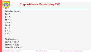
Solution Found:
D = 7
E = 5
M = 1
N = 6
O = 0
R = 8
S = 9
Y = 2
Verification:
SEND = 9567
MORE = 1085
MONEY = 10652
95.
Types of Constraintsin CSP
Artificial Intelligence – Unit-II Mr. R. N. Kankrale Department of Information Technology
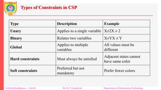
Type Description Example
Unary Applies to a single variable X≠2X ≠ 2
Binary Relates two variables X≠YX ≠ Y
Global
Applies to multiple
variables
All values must be
different
Hard constraints Must always be satisfied
Adjacent states cannot
have same color
Soft constraints
Preferred but not
mandatory
Prefer fewer colors
96.
CSP Solving Techniques
ArtificialIntelligence – Unit-II Mr. R. N. Kankrale Department of Information Technology
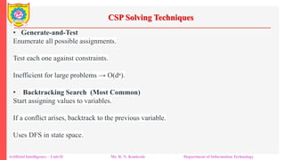
• Generate-and-Test
Enumerate all possible assignments.
Test each one against constraints.
Inefficient for large problems → O(dⁿ).
• Backtracking Search (Most Common)
Start assigning values to variables.
If a conflict arises, backtrack to the previous variable.
Uses DFS in state space.
97.
Real-Life Applications ofCSP
Artificial Intelligence – Unit-II Mr. R. N. Kankrale Department of Information Technology
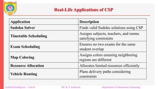
Application Description
Sudoku Solver Finds valid Sudoku solutions using CSP
Timetable Scheduling
Assigns subjects, teachers, and rooms
satisfying constraints
Exam Scheduling
Ensures no two exams for the same
student overlap
Map Coloring
Assigns colors ensuring neighboring
regions are different
Resource Allocation Allocates limited resources efficiently
Vehicle Routing
Plans delivery paths considering
constraints
98.
Constraint Satisfaction Problems(CSP) in Artificial Intelligence
Artificial Intelligence – Unit-II Mr. R. N. Kankrale Department of Information Technology
There are mainly three basic components in the constraint satisfaction
problem:
Variables: The things that need to be determined are variables. Variables in a
CSP are the objects that must have values assigned to them in order to satisfy a
particular set of constraints. Boolean, integer, and categorical variables are just a
few examples of the various types of variables, for instance, could stand in for
the many puzzle cells that need to be filled with numbers in a sudoku puzzle.
Domains: The range of potential values that a variable can have is represented
by domains. Depending on the issue, a domain may be finite or limitless. For
instance, in Sudoku, the set of numbers from 1 to 9 can serve as the domain of a
variable representing a problem cell.
99.
Constraint Satisfaction Problems(CSP) in Artificial Intelligence
Artificial Intelligence – Unit-II Mr. R. N. Kankrale Department of Information Technology
Constraints: The guidelines that control how variables relate to one another are
known as constraints. Constraints in a CSP define the ranges of possible values
for variables. Unary constraints, binary constraints, and higher-order constraints
are only a few examples of the various sorts of constraints. For instance, in a
sudoku problem, the restrictions might be that each row, column, and 3×3 box
can only have one instance of each number from 1 to 9.
100.
Constraint Satisfaction Problems(CSP) in Artificial Intelligence
Artificial Intelligence – Unit-II Mr. R. N. Kankrale Department of Information Technology
Constraint Satisfaction Problems (CSP) representation:
•The finite set of variables V1, V2, V3 ……………..Vn.
•Non-empty domain for every single variable D1, D2, D3 …………..Dn.
•The finite set of constraints C1, C2 …….…, Cm.
• where each constraint Ci restricts the possible values for variables,
• e.g., V1 ≠ V2
• Each constraint Ci is a pair <scope, relation>
• Example: <(V1, V2), V1 not equal to V2>
• Scope = set of variables that participate in constraint.
• Relation = list of valid variable value combinations.
• There might be a clear list of permitted combinations. Perhaps a relation that is
abstract and that allows for membership testing and listing.