DAGs for Common Biases
M. Maria Glymour
Department of Epidemiology and Biostatistics
University of California, San Francisco
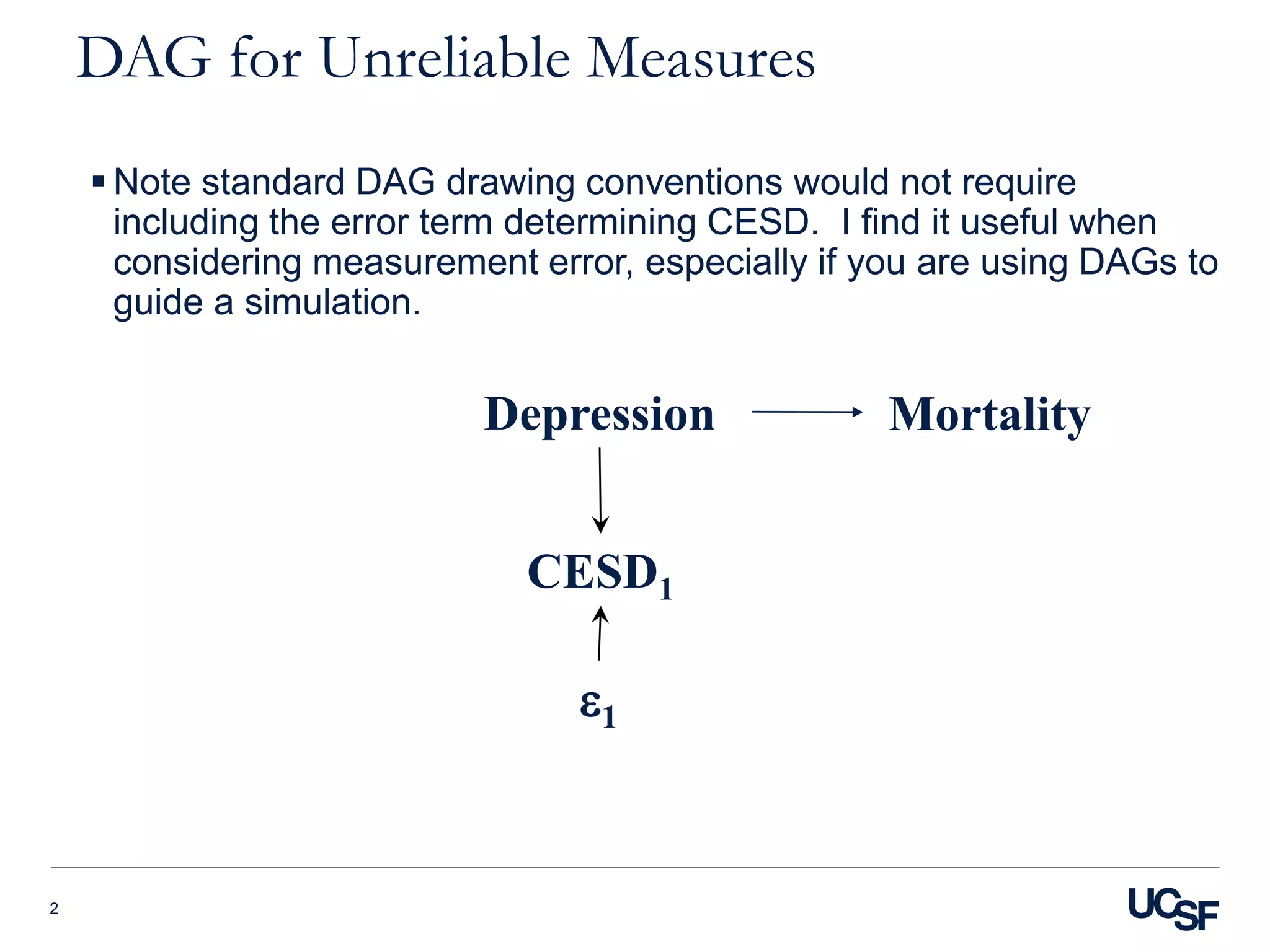
DAG for Unreliable Measures
2
Depression Mortality
CESD1
e1
ī‚§ Note standard DAG drawing conventions would not require
including the error term determining CESD. I find it useful when
considering measurement error, especially if you are using DAGs to
guide a simulation.
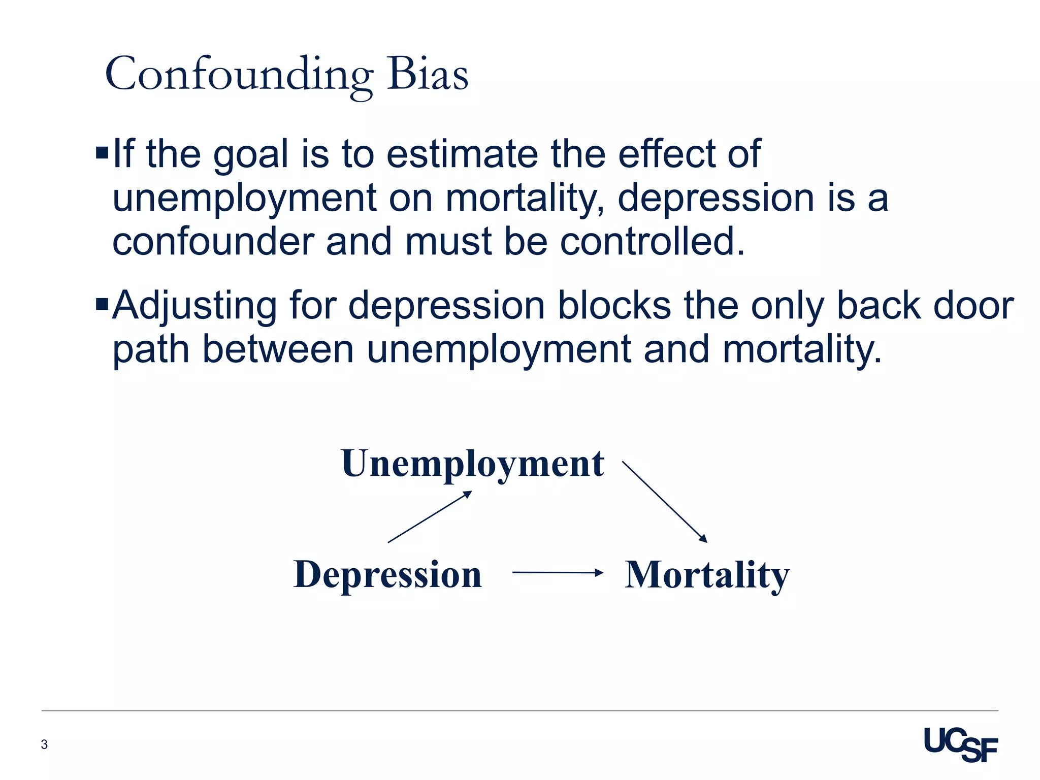
Confounding Bias
ī‚§If the goal is to estimate the effect of
unemployment on mortality, depression is a
confounder and must be controlled.
ī‚§Adjusting for depression blocks the only back door
path between unemployment and mortality.
3
Depression Mortality
Unemployment
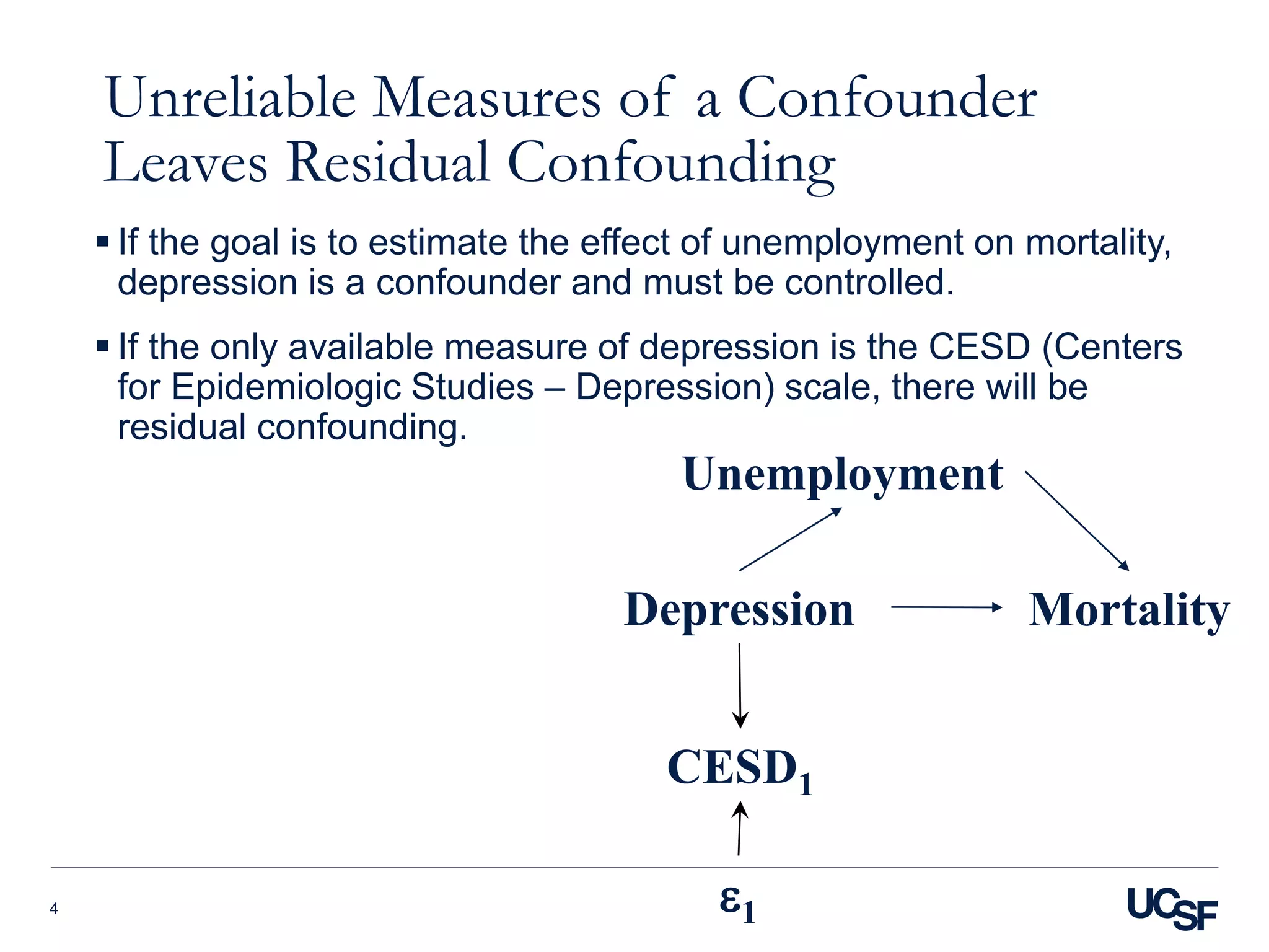
Unreliable Measures of a Confounder
Leaves Residual Confounding
ī‚§ If the goal is to estimate the effect of unemployment on mortality,
depression is a confounder and must be controlled.
ī‚§ If the only available measure of depression is the CESD (Centers
for Epidemiologic Studies – Depression) scale, there will be
residual confounding.
4
Depression Mortality
CESD1
e1
Unemployment
Unreliable Measures in Analyses of Change
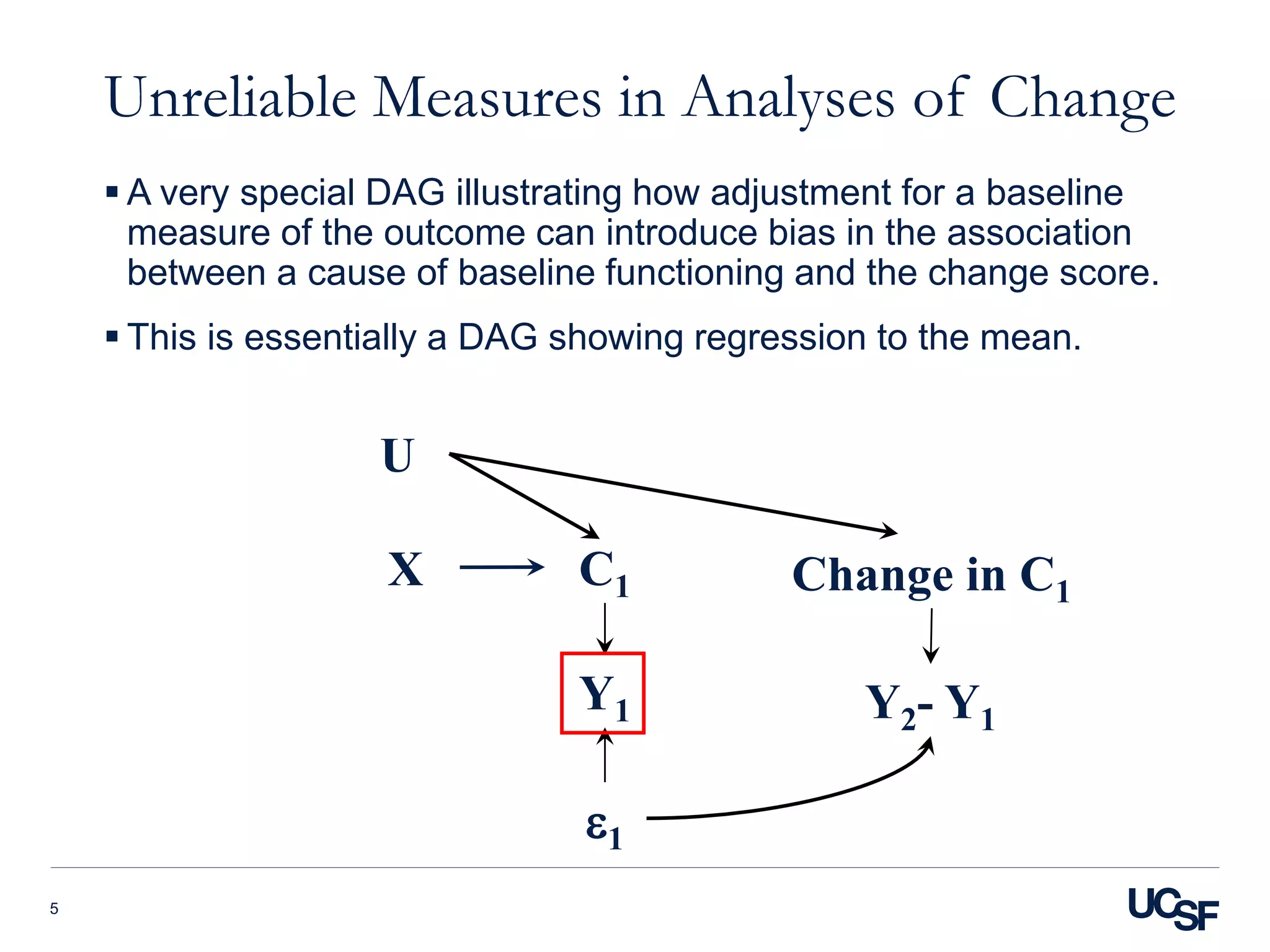
ī‚§ A very special DAG illustrating how adjustment for a baseline
measure of the outcome can introduce bias in the association
between a cause of baseline functioning and the change score.
ī‚§ This is essentially a DAG showing regression to the mean.
5
X C1 Change in C1
Y1
e1
U
Y2- Y1
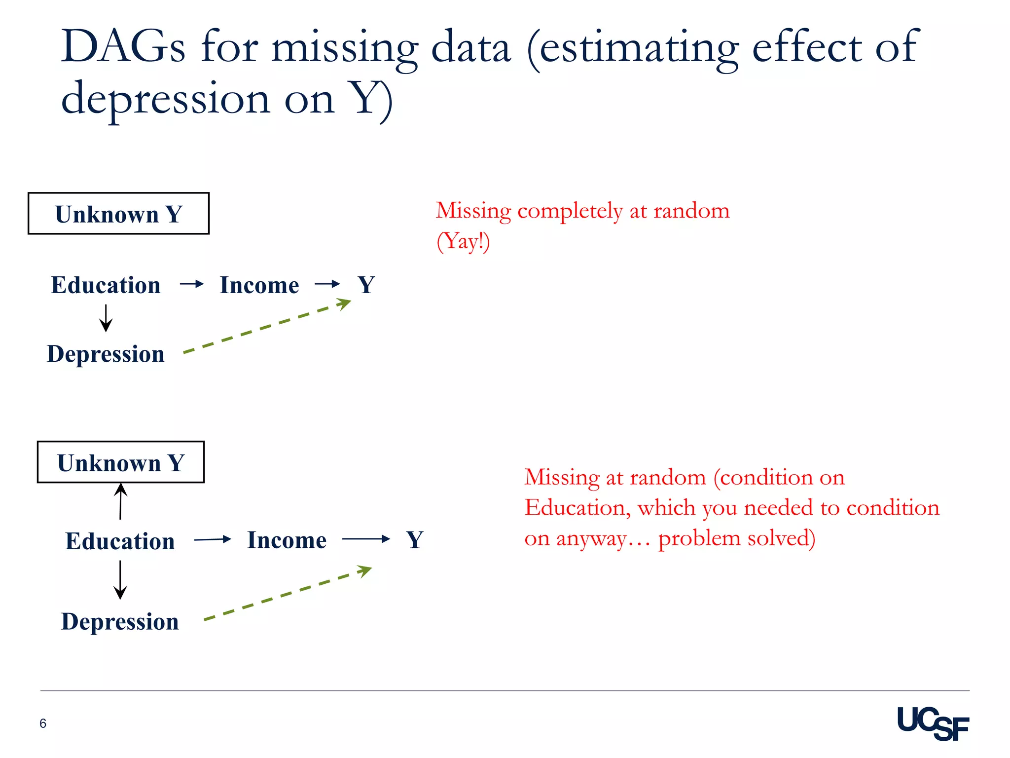
DAGs for missing data (estimating effect of
depression on Y)
6
Education Income
Depression
Y
Unknown Y Missing completely at random
(Yay!)
Education Income
Depression
Y
Unknown Y
Missing at random (condition on
Education, which you needed to condition
on anywayâ€Ļ problem solved)
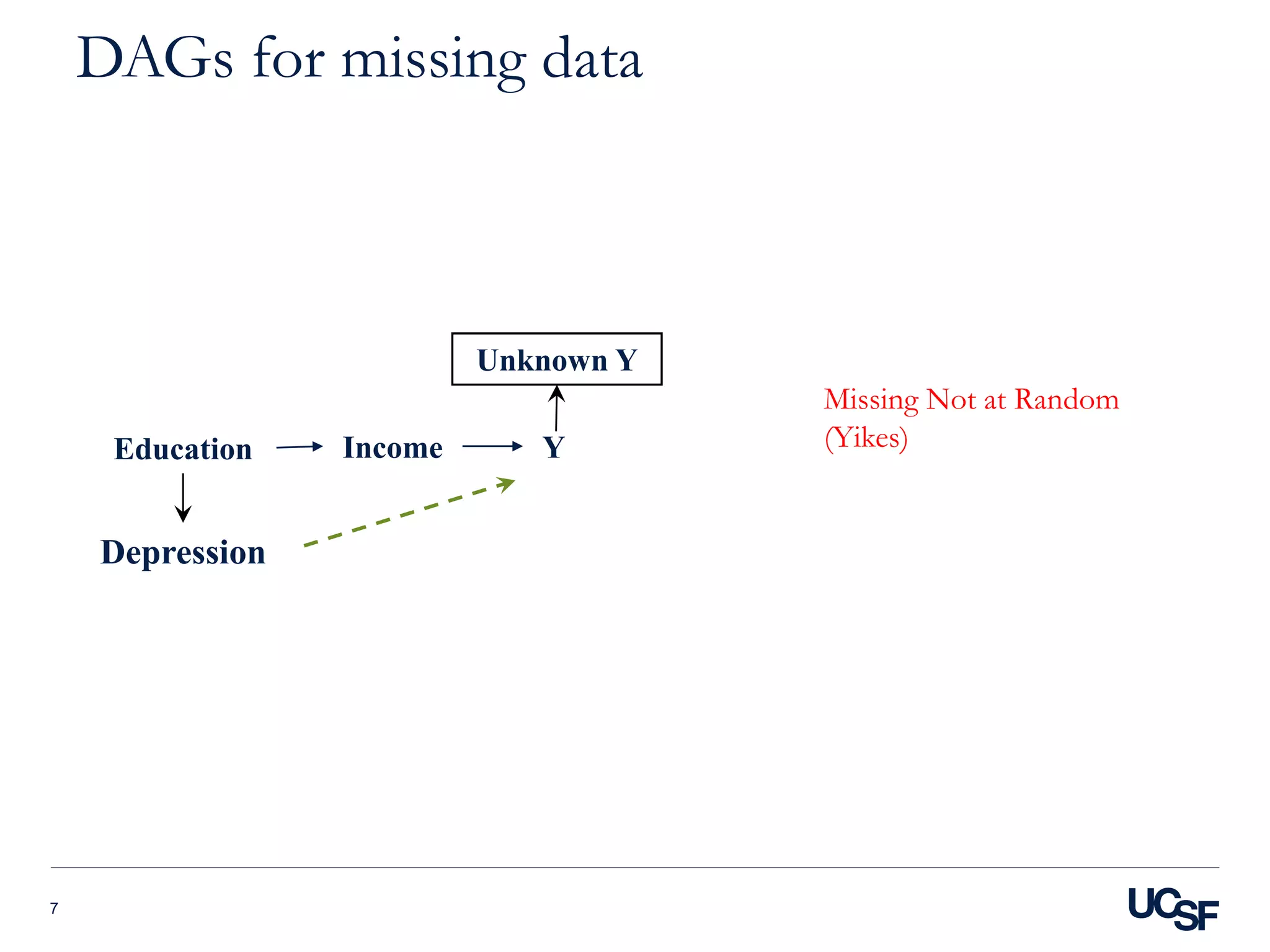
DAGs for missing data
7
Education Income
Depression
Y
Unknown Y
Missing Not at Random
(Yikes)
Immortal time bias
ī‚§ Bias occurs when there is “A span of time in the observation or
follow-up period of a cohort during which the outcome under study
could not have occurred.”
ī‚§ Example: comparing effect of heart transplant receipt on survival
time, beginning follow up at the time patient is placed on the wait list.
The time from wait list placement to receipt of the transplant is
“immortal time” for any analysis conducted among transplant
recipients in that, had they died during this period before the
transplant, they would not have received the transplant (organ
donation rules being limited to living recipients).
ī‚§ Sometimes called “survivor treatment selection bias” but that is a
very confusing label.
ī‚§ There are several variations that might be referred to as immortal
time bias but correspond with somewhat distinct causal structures.
DAGs for the most innocuous variant of
immortal time bias
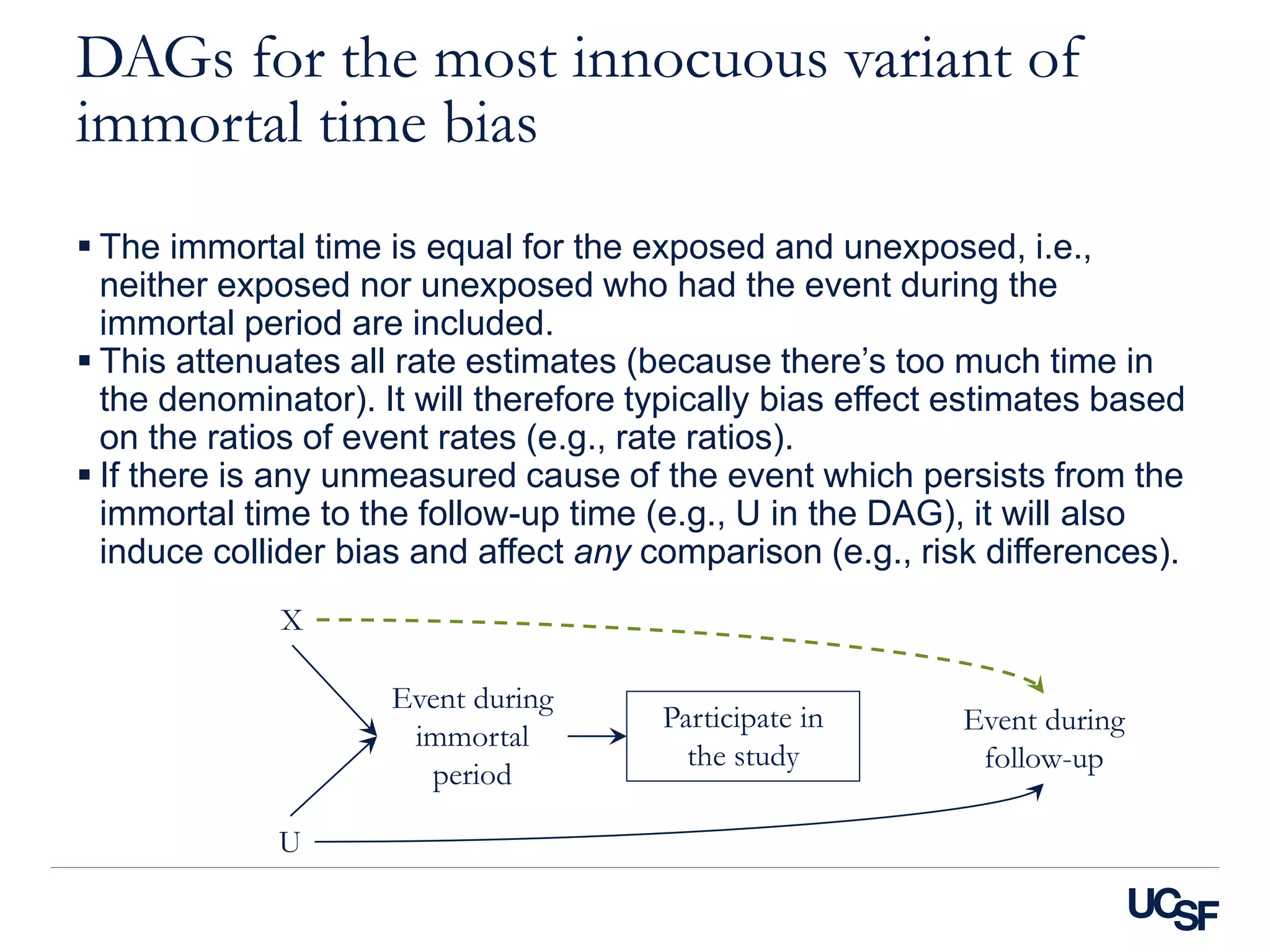
ī‚§ The immortal time is equal for the exposed and unexposed, i.e.,
neither exposed nor unexposed who had the event during the
immortal period are included.
ī‚§ This attenuates all rate estimates (because there’s too much time in
the denominator). It will therefore typically bias effect estimates based
on the ratios of event rates (e.g., rate ratios).
ī‚§ If there is any unmeasured cause of the event which persists from the
immortal time to the follow-up time (e.g., U in the DAG), it will also
induce collider bias and affect any comparison (e.g., risk differences).
X
Event during
immortal
period
Event during
follow-up
Participate in
the study
U
DAGs for the most innocuous variant of
immortal time bias
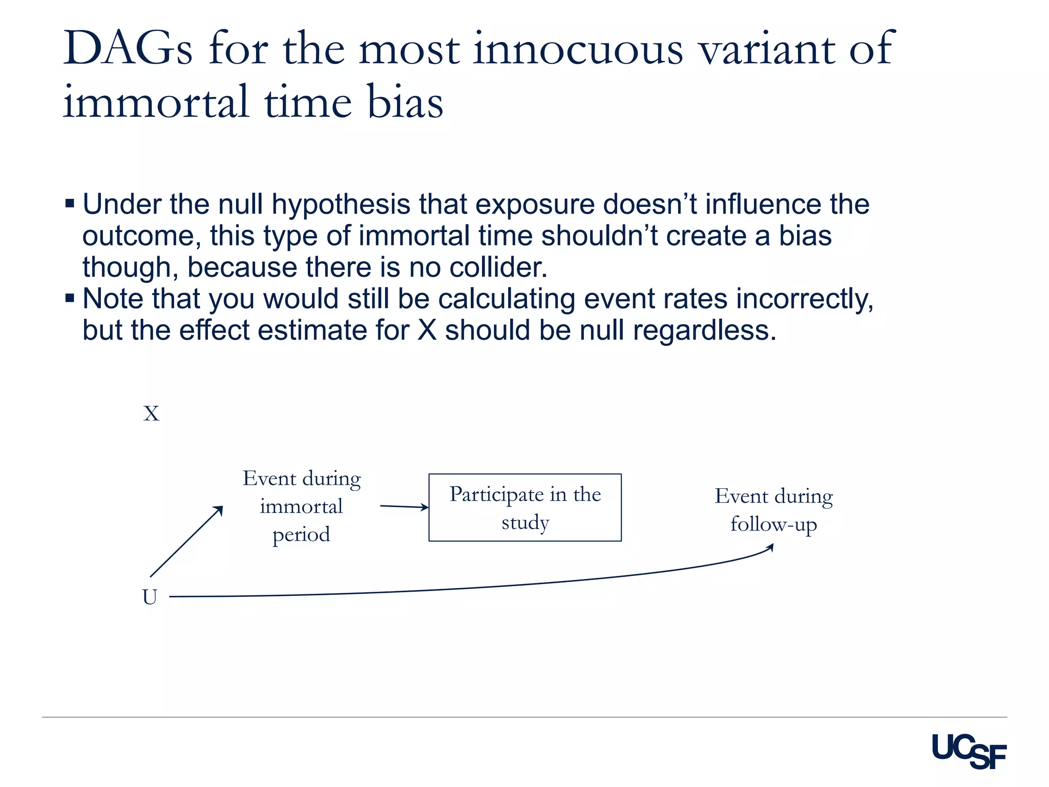
ī‚§ Under the null hypothesis that exposure doesn’t influence the
outcome, this type of immortal time shouldn’t create a bias
though, because there is no collider.
ī‚§ Note that you would still be calculating event rates incorrectly,
but the effect estimate for X should be null regardless.
X
Event during
immortal
period
Event during
follow-up
Participate in the
study
U
DAGs for the worst variant of immortal
time bias
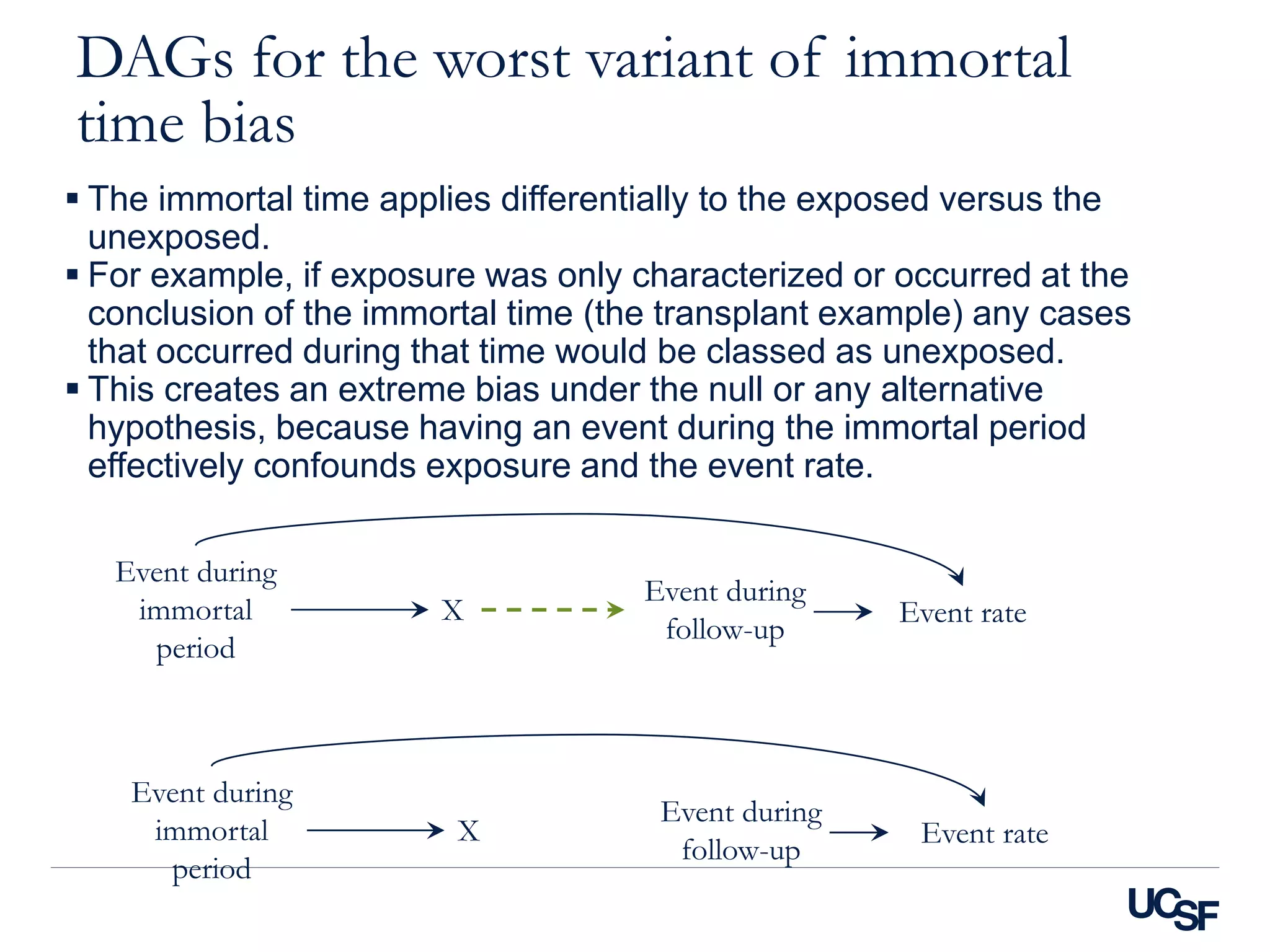
ī‚§ The immortal time applies differentially to the exposed versus the
unexposed.
ī‚§ For example, if exposure was only characterized or occurred at the
conclusion of the immortal time (the transplant example) any cases
that occurred during that time would be classed as unexposed.
ī‚§ This creates an extreme bias under the null or any alternative
hypothesis, because having an event during the immortal period
effectively confounds exposure and the event rate.
X
Event during
immortal
period
Event during
follow-up
Event rate
X
Event during
immortal
period
Event during
follow-up
Event rate
DAGs for an especially seductive variant of
immortal time bias
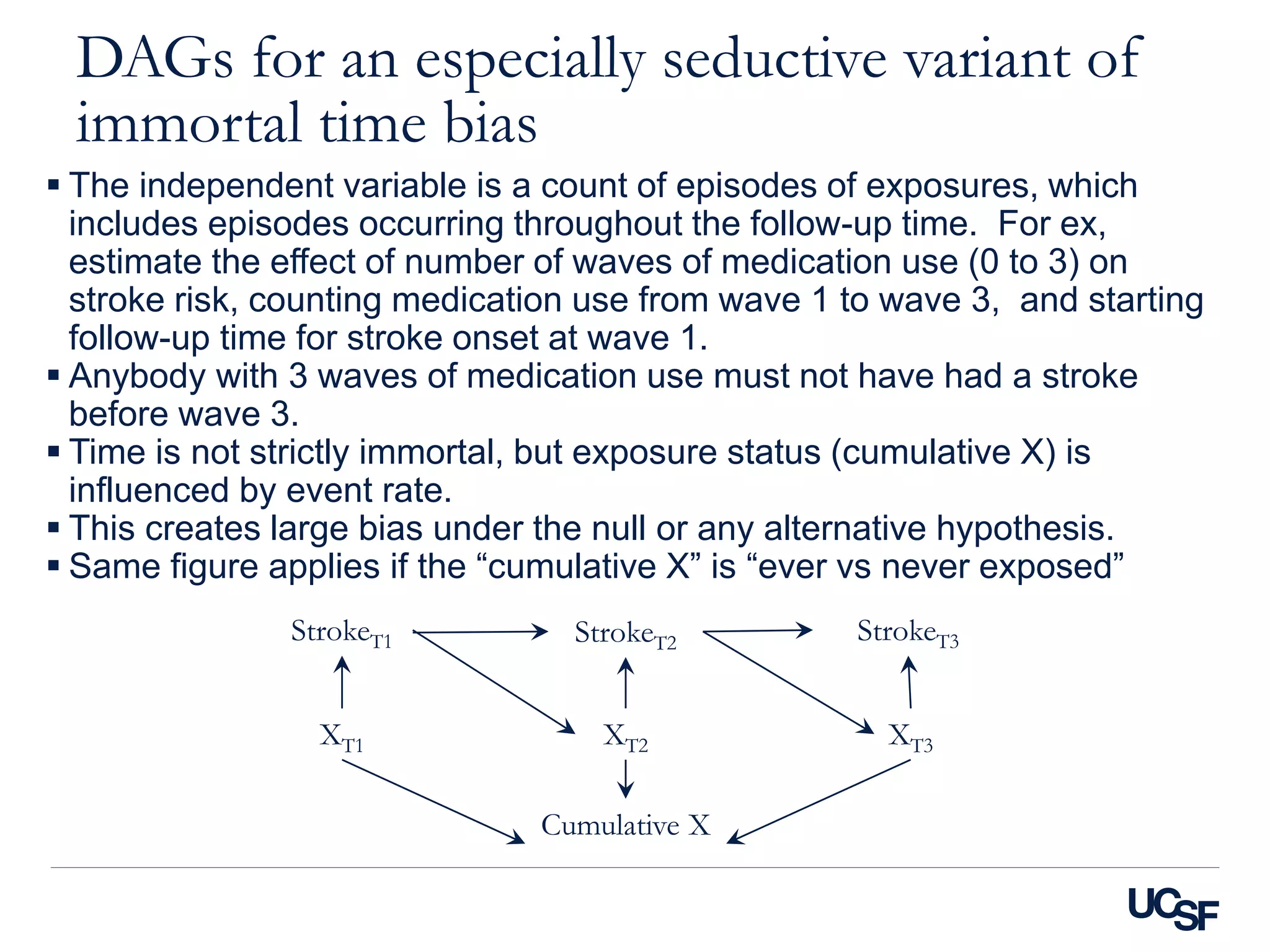
ī‚§ The independent variable is a count of episodes of exposures, which
includes episodes occurring throughout the follow-up time. For ex,
estimate the effect of number of waves of medication use (0 to 3) on
stroke risk, counting medication use from wave 1 to wave 3, and starting
follow-up time for stroke onset at wave 1.
ī‚§ Anybody with 3 waves of medication use must not have had a stroke
before wave 3.
ī‚§ Time is not strictly immortal, but exposure status (cumulative X) is
influenced by event rate.
ī‚§ This creates large bias under the null or any alternative hypothesis.
ī‚§ Same figure applies if the “cumulative X” is “ever vs never exposed”
XT1
StrokeT1 StrokeT2
XT2
StrokeT3
XT3
Cumulative X
M YX
U
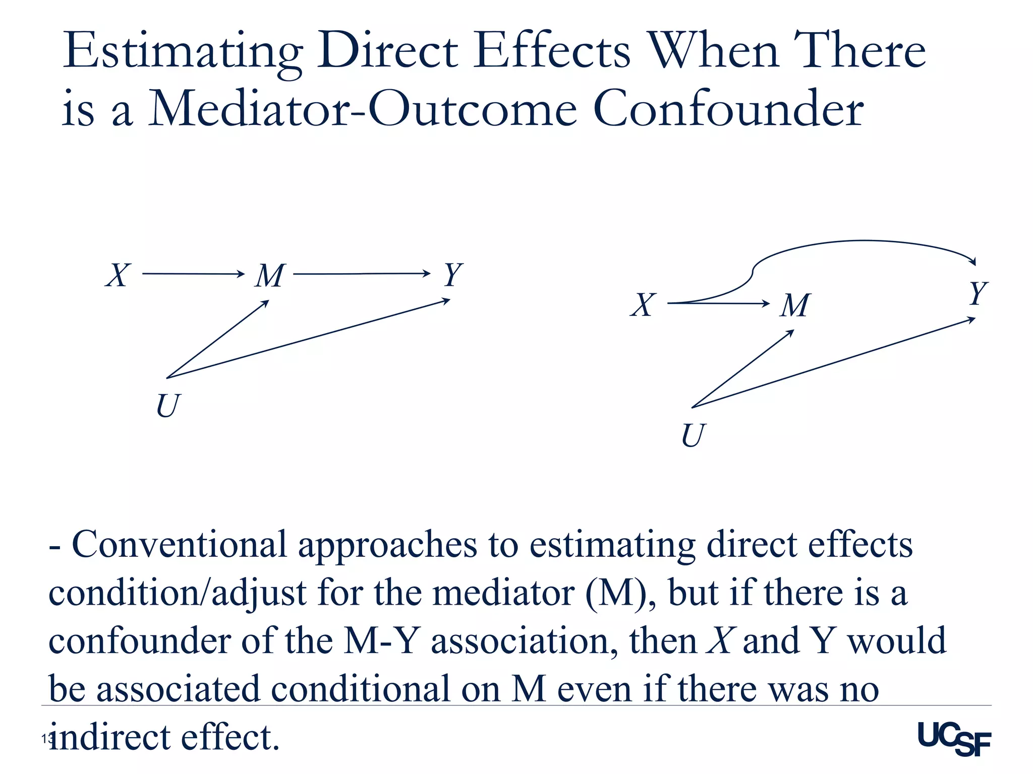
Estimating Direct Effects When There
is a Mediator-Outcome Confounder
13
- Conventional approaches to estimating direct effects
condition/adjust for the mediator (M), but if there is a
confounder of the M-Y association, then X and Y would
be associated conditional on M even if there was no
indirect effect.
M YX
U
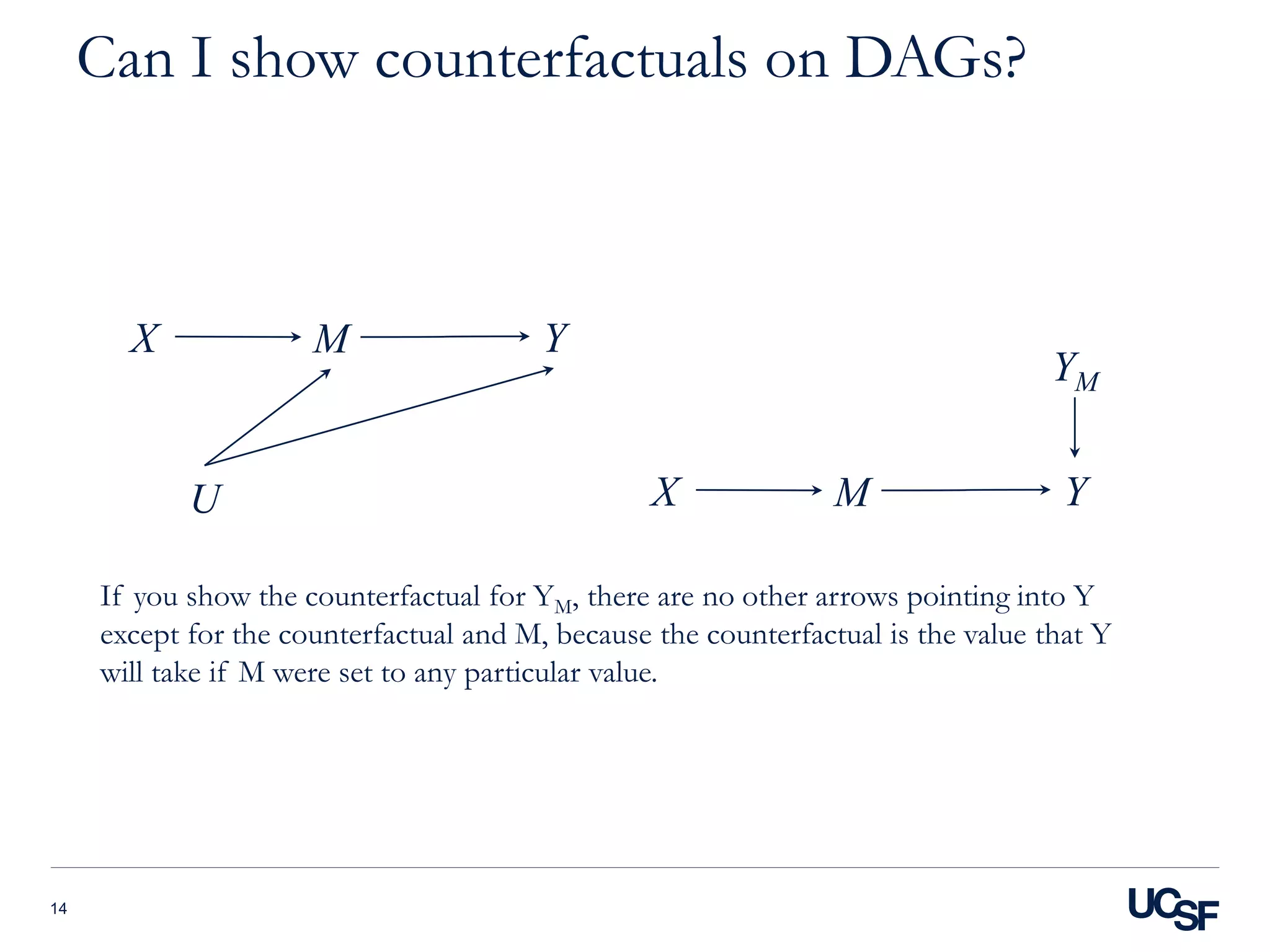
Can I show counterfactuals on DAGs?
14
M YX
YM
If you show the counterfactual for YM, there are no other arrows pointing into Y
except for the counterfactual and M, because the counterfactual is the value that Y
will take if M were set to any particular value.
M YX
U
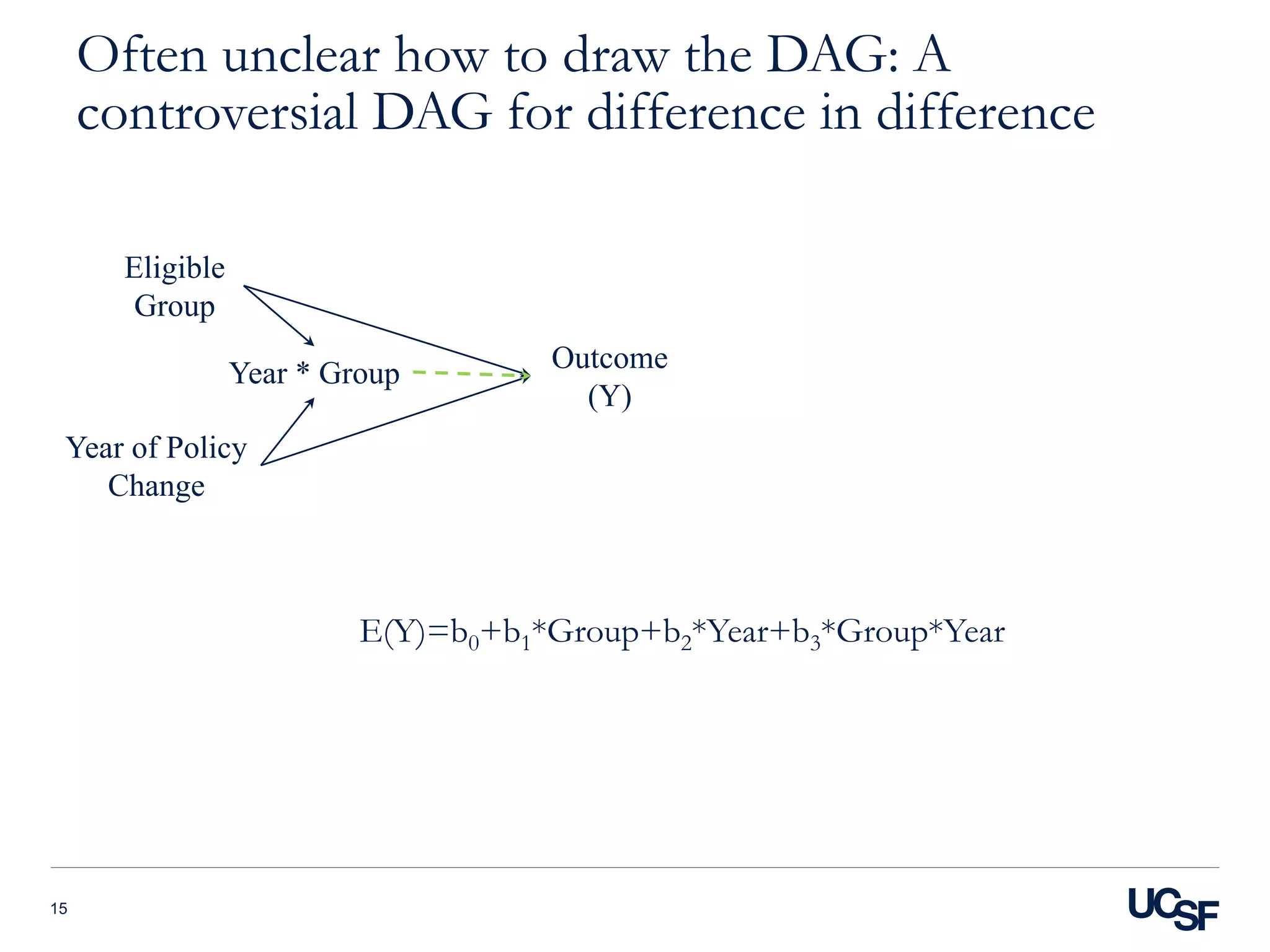
Often unclear how to draw the DAG: A
controversial DAG for difference in difference
15
Year * Group Outcome
(Y)
Eligible
Group
Year of Policy
Change
E(Y)=b0+b1*Group+b2*Year+b3*Group*Year
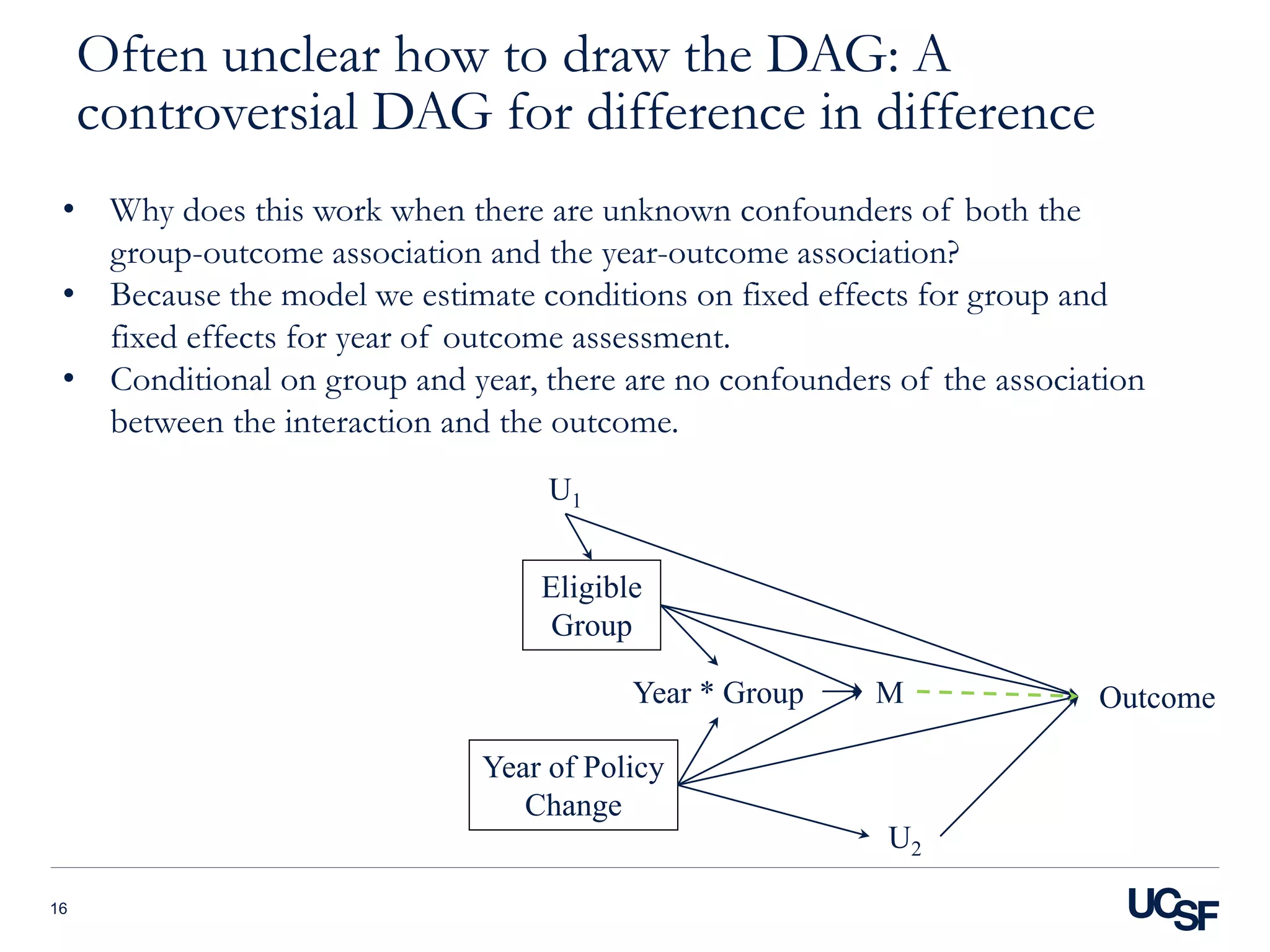
Often unclear how to draw the DAG: A
controversial DAG for difference in difference
16
Year * Group Outcome
Eligible
Group
Year of Policy
Change
M
U1
U2
â€ĸ Why does this work when there are unknown confounders of both the
group-outcome association and the year-outcome association?
â€ĸ Because the model we estimate conditions on fixed effects for group and
fixed effects for year of outcome assessment.
â€ĸ Conditional on group and year, there are no confounders of the association
between the interaction and the outcome.
17
PhD Program in
Epidemiology and
Translational
Science
https://epibiostat.ucsf.edu/doctoral-program-
epidemiology-translational-science

Da gs for_commonbiases2

  • 1.
    DAGs for CommonBiases M. Maria Glymour Department of Epidemiology and Biostatistics University of California, San Francisco
  • 2.
    DAG for UnreliableMeasures 2 Depression Mortality CESD1 e1 ī‚§ Note standard DAG drawing conventions would not require including the error term determining CESD. I find it useful when considering measurement error, especially if you are using DAGs to guide a simulation.
  • 3.
    Confounding Bias ī‚§If thegoal is to estimate the effect of unemployment on mortality, depression is a confounder and must be controlled. ī‚§Adjusting for depression blocks the only back door path between unemployment and mortality. 3 Depression Mortality Unemployment
  • 4.
    Unreliable Measures ofa Confounder Leaves Residual Confounding ī‚§ If the goal is to estimate the effect of unemployment on mortality, depression is a confounder and must be controlled. ī‚§ If the only available measure of depression is the CESD (Centers for Epidemiologic Studies – Depression) scale, there will be residual confounding. 4 Depression Mortality CESD1 e1 Unemployment
  • 5.
    Unreliable Measures inAnalyses of Change ī‚§ A very special DAG illustrating how adjustment for a baseline measure of the outcome can introduce bias in the association between a cause of baseline functioning and the change score. ī‚§ This is essentially a DAG showing regression to the mean. 5 X C1 Change in C1 Y1 e1 U Y2- Y1
  • 6.
    DAGs for missingdata (estimating effect of depression on Y) 6 Education Income Depression Y Unknown Y Missing completely at random (Yay!) Education Income Depression Y Unknown Y Missing at random (condition on Education, which you needed to condition on anywayâ€Ļ problem solved)
  • 7.
    DAGs for missingdata 7 Education Income Depression Y Unknown Y Missing Not at Random (Yikes)
  • 8.
    Immortal time bias ī‚§Bias occurs when there is “A span of time in the observation or follow-up period of a cohort during which the outcome under study could not have occurred.” ī‚§ Example: comparing effect of heart transplant receipt on survival time, beginning follow up at the time patient is placed on the wait list. The time from wait list placement to receipt of the transplant is “immortal time” for any analysis conducted among transplant recipients in that, had they died during this period before the transplant, they would not have received the transplant (organ donation rules being limited to living recipients). ī‚§ Sometimes called “survivor treatment selection bias” but that is a very confusing label. ī‚§ There are several variations that might be referred to as immortal time bias but correspond with somewhat distinct causal structures.
  • 9.
    DAGs for themost innocuous variant of immortal time bias ī‚§ The immortal time is equal for the exposed and unexposed, i.e., neither exposed nor unexposed who had the event during the immortal period are included. ī‚§ This attenuates all rate estimates (because there’s too much time in the denominator). It will therefore typically bias effect estimates based on the ratios of event rates (e.g., rate ratios). ī‚§ If there is any unmeasured cause of the event which persists from the immortal time to the follow-up time (e.g., U in the DAG), it will also induce collider bias and affect any comparison (e.g., risk differences). X Event during immortal period Event during follow-up Participate in the study U
  • 10.
    DAGs for themost innocuous variant of immortal time bias ī‚§ Under the null hypothesis that exposure doesn’t influence the outcome, this type of immortal time shouldn’t create a bias though, because there is no collider. ī‚§ Note that you would still be calculating event rates incorrectly, but the effect estimate for X should be null regardless. X Event during immortal period Event during follow-up Participate in the study U
  • 11.
    DAGs for theworst variant of immortal time bias ī‚§ The immortal time applies differentially to the exposed versus the unexposed. ī‚§ For example, if exposure was only characterized or occurred at the conclusion of the immortal time (the transplant example) any cases that occurred during that time would be classed as unexposed. ī‚§ This creates an extreme bias under the null or any alternative hypothesis, because having an event during the immortal period effectively confounds exposure and the event rate. X Event during immortal period Event during follow-up Event rate X Event during immortal period Event during follow-up Event rate
  • 12.
    DAGs for anespecially seductive variant of immortal time bias ī‚§ The independent variable is a count of episodes of exposures, which includes episodes occurring throughout the follow-up time. For ex, estimate the effect of number of waves of medication use (0 to 3) on stroke risk, counting medication use from wave 1 to wave 3, and starting follow-up time for stroke onset at wave 1. ī‚§ Anybody with 3 waves of medication use must not have had a stroke before wave 3. ī‚§ Time is not strictly immortal, but exposure status (cumulative X) is influenced by event rate. ī‚§ This creates large bias under the null or any alternative hypothesis. ī‚§ Same figure applies if the “cumulative X” is “ever vs never exposed” XT1 StrokeT1 StrokeT2 XT2 StrokeT3 XT3 Cumulative X
  • 13.
    M YX U Estimating DirectEffects When There is a Mediator-Outcome Confounder 13 - Conventional approaches to estimating direct effects condition/adjust for the mediator (M), but if there is a confounder of the M-Y association, then X and Y would be associated conditional on M even if there was no indirect effect. M YX U
  • 14.
    Can I showcounterfactuals on DAGs? 14 M YX YM If you show the counterfactual for YM, there are no other arrows pointing into Y except for the counterfactual and M, because the counterfactual is the value that Y will take if M were set to any particular value. M YX U
  • 15.
    Often unclear howto draw the DAG: A controversial DAG for difference in difference 15 Year * Group Outcome (Y) Eligible Group Year of Policy Change E(Y)=b0+b1*Group+b2*Year+b3*Group*Year
  • 16.
    Often unclear howto draw the DAG: A controversial DAG for difference in difference 16 Year * Group Outcome Eligible Group Year of Policy Change M U1 U2 â€ĸ Why does this work when there are unknown confounders of both the group-outcome association and the year-outcome association? â€ĸ Because the model we estimate conditions on fixed effects for group and fixed effects for year of outcome assessment. â€ĸ Conditional on group and year, there are no confounders of the association between the interaction and the outcome.
  • 17.
    17 PhD Program in Epidemiologyand Translational Science https://epibiostat.ucsf.edu/doctoral-program- epidemiology-translational-science