ADVANCING SMOOTHLY
CRUISE CONTROL
CRUISE CONTROL
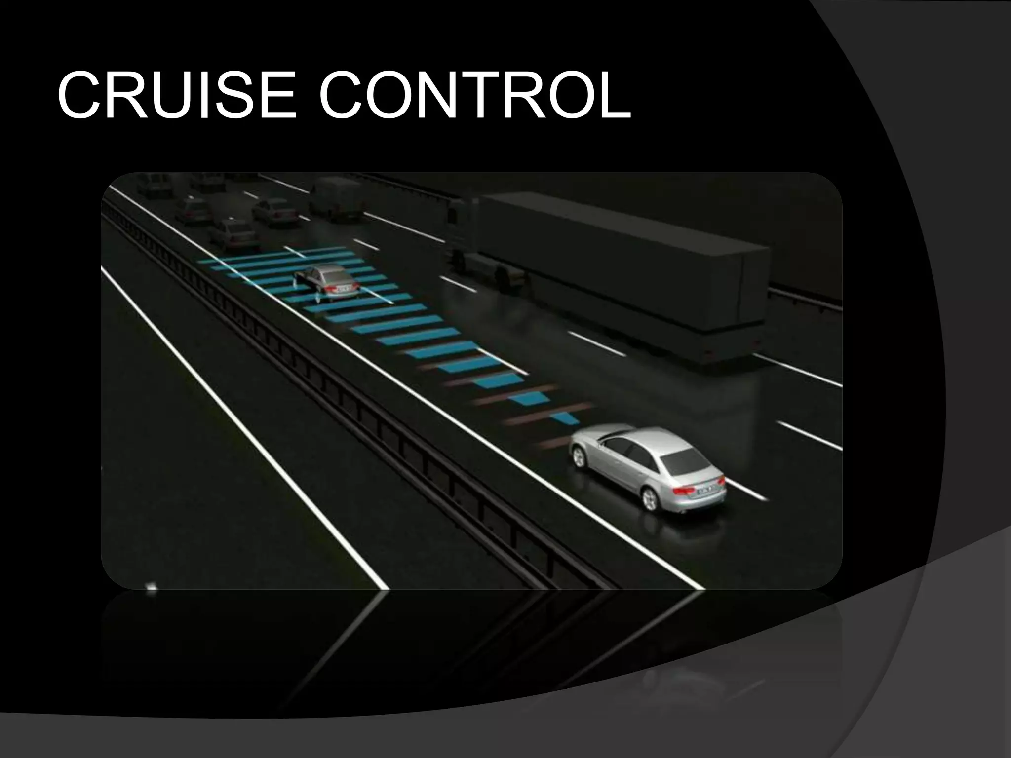
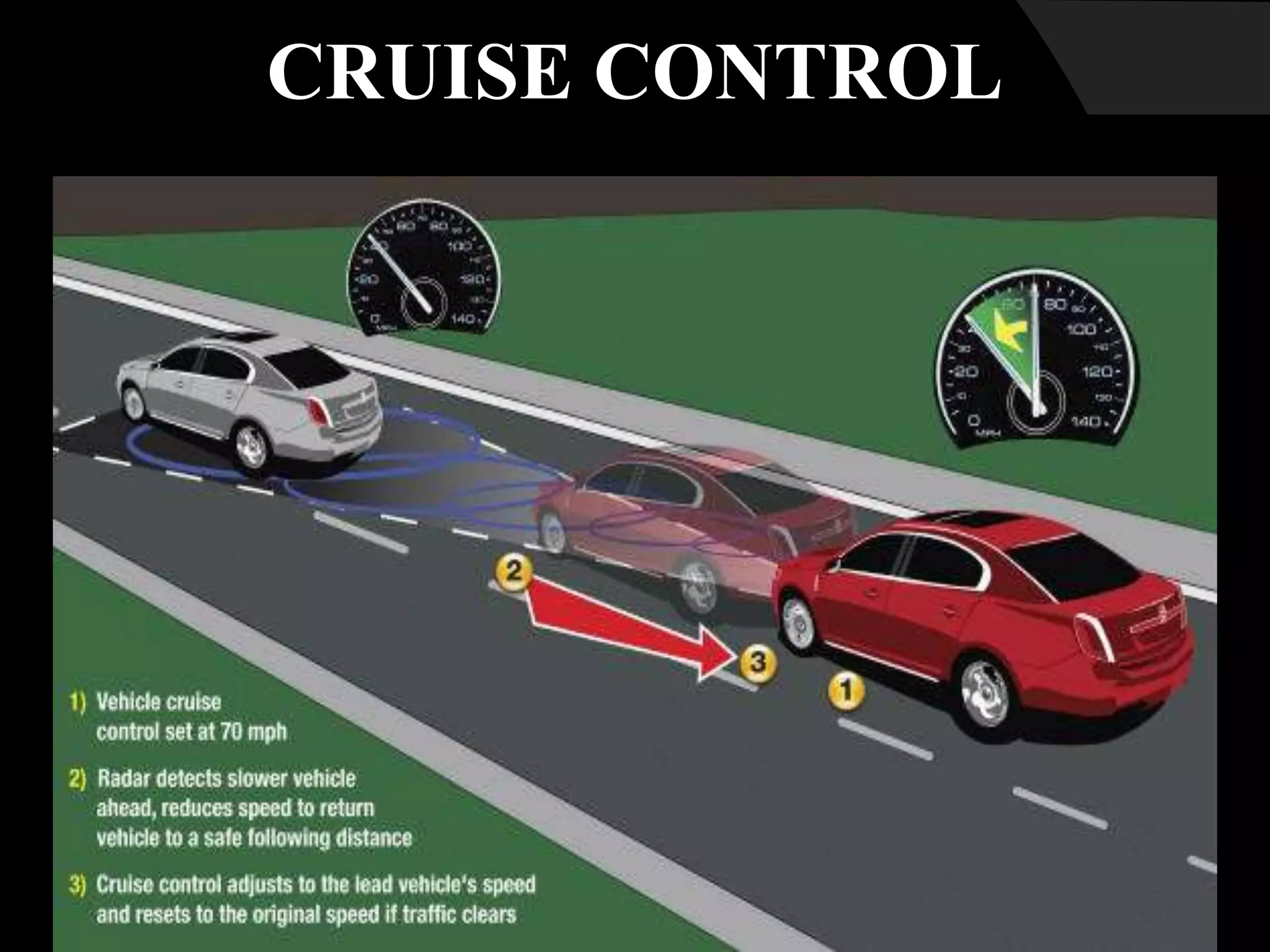
 Cruise control (speed control, auto-cruise
or tempomat) is a system that automatically
controls the speed of a motor vehicle. The system
takes over the throttle of the car to maintain a
steady speed as set by the driver.
CRUISE CONTROL
SYSTEM MODELLING
 feedback control system
 purpose is to maintain a constant vehicle
speed despite external disturbances, such
as changes in wind or road grade.
 accomplished by
i. measuring the vehicle speed
ii. comparing it to the desired or reference speed
iii. automatically adjusting the throttle according
to a control law
PHYSICAL SETUP: FBD
bv u
 Mass m
 Control force u
 Resistive forces bv
 Vehicle velocity v
 u = force generated at the road/tire
interface
 we will assume that :
i. u can be controlled directly
ii. the dynamics of the
powertrain, tires, etc are 0
iii. bv, due to rolling resistance and wind
drag varies linearly with the vehicle
velocity, v, and act in the direction
opposite the vehicle's motion
FIRST ORDER EQUATION
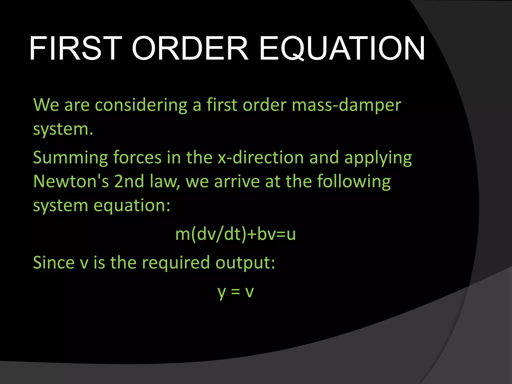
We are considering a first order mass-damper
system.
Summing forces in the x-direction and applying
Newton's 2nd law, we arrive at the following
system equation:
m(dv/dt)+bv=u
Since v is the required output:
y = v
TRANSFER FUNCTION
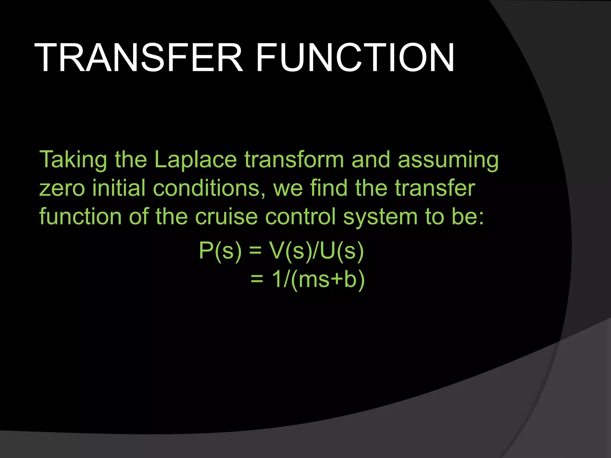
Taking the Laplace transform and assuming
zero initial conditions, we find the transfer
function of the cruise control system to be:
P(s) = V(s)/U(s)
= 1/(ms+b)
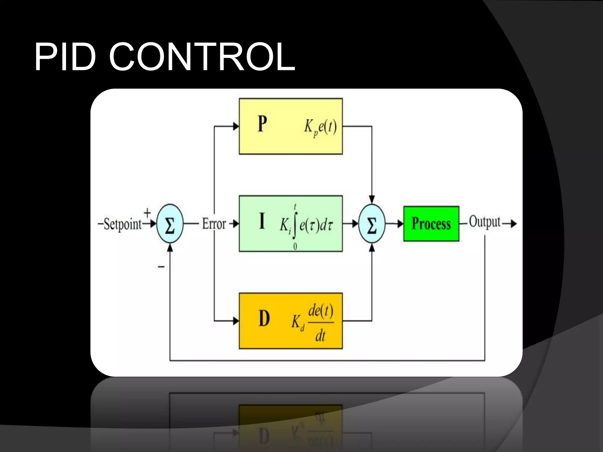
PID CONTROL
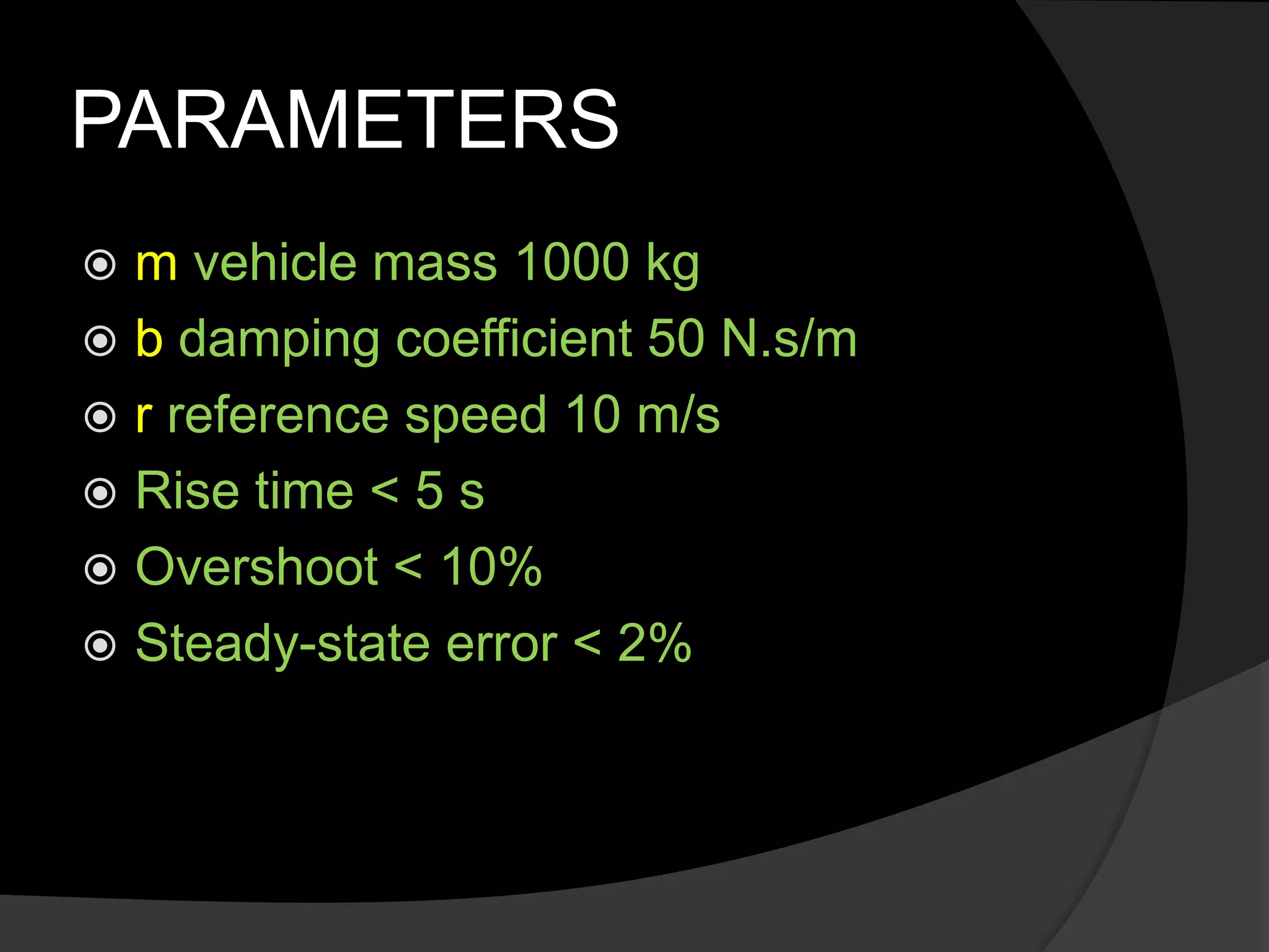
PARAMETERS
 m vehicle mass 1000 kg
 b damping coefficient 50 N.s/m
 r reference speed 10 m/s
 Rise time < 5 s
 Overshoot < 10%
 Steady-state error < 2%
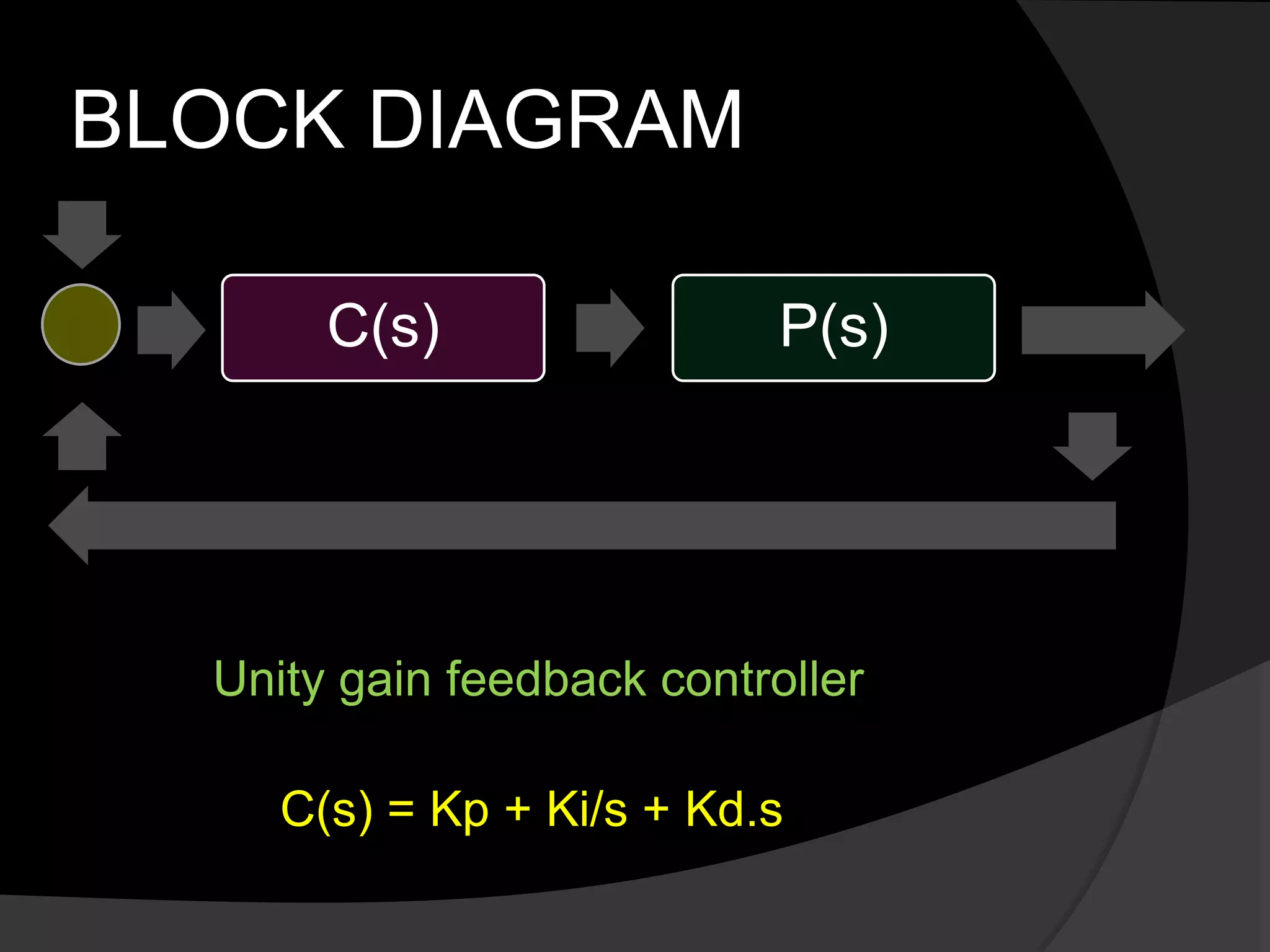
BLOCK DIAGRAM
C(s) P(s)
Unity gain feedback controller
C(s) = Kp + Ki/s + Kd.s
PROPORTIONAL
CONTROL
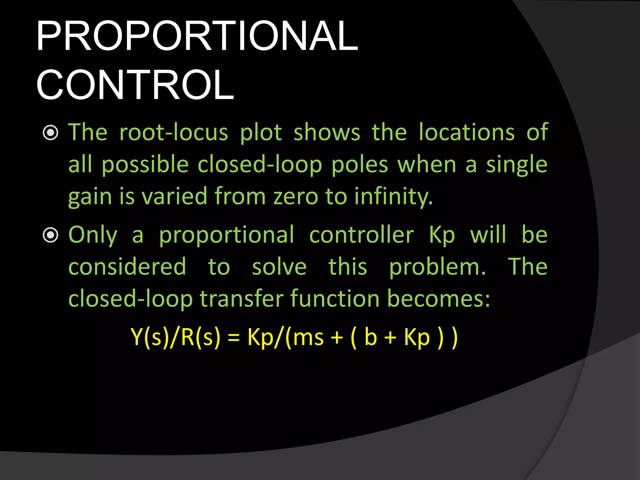
 The root-locus plot shows the locations of
all possible closed-loop poles when a single
gain is varied from zero to infinity.
 Only a proportional controller Kp will be
considered to solve this problem. The
closed-loop transfer function becomes:
Y(s)/R(s) = Kp/(ms + ( b + Kp ) )
PROPORTIONAL
CONTROL
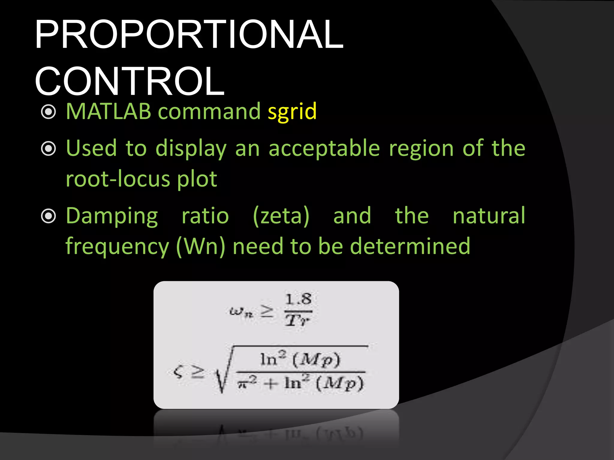
 MATLAB command sgrid
 Used to display an acceptable region of the
root-locus plot
 Damping ratio (zeta) and the natural
frequency (Wn) need to be determined
PROPORTIONAL
CONTROL
PROPORTIONAL
CONTROL
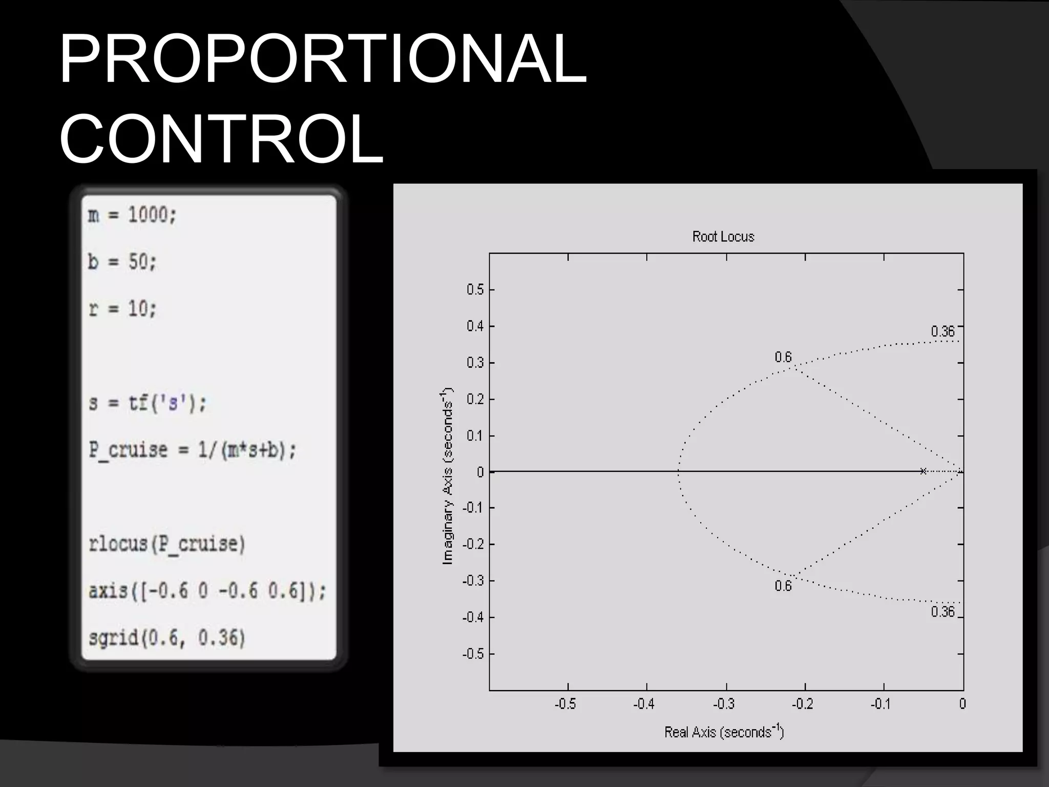
 We can then find a gain to place the closed-
loop poles in the desired region by
employing the rlocfind command
 specific loop gain
[Kp,poles]=rlocfind(P_cruise)
 In between the dotted lines (zeta > 0.6) and
outside the semi-ellipse (wn > 0.36)
LAG CONTROLLER
 With the gain Kp being the only functional
gain and Ki and Kd being zero, the rise time
and the overshoot criteria have been met
 A steady-state error of more than 10%
remains
 To reduce the steady-state error, a lag
controller is added to the system
LAG CONTROLLER
 To reduce the steady-state error, a lag
controller will be added to the system.
 A pole and a zero, not too distant spacing-
wise are introduced i.e:
LAG CONTROLLER
 With the gain Kp being the only functional
gain and Ki and Kd being zero, the rise time
and the overshoot criteria have been met
 A steady-state error of more than 10%
remains
 To reduce the steady-state error, a lag
controller is added to the system
 the steady-state error will be reduced by a
factor of zo/po
LAG CONTROLLER
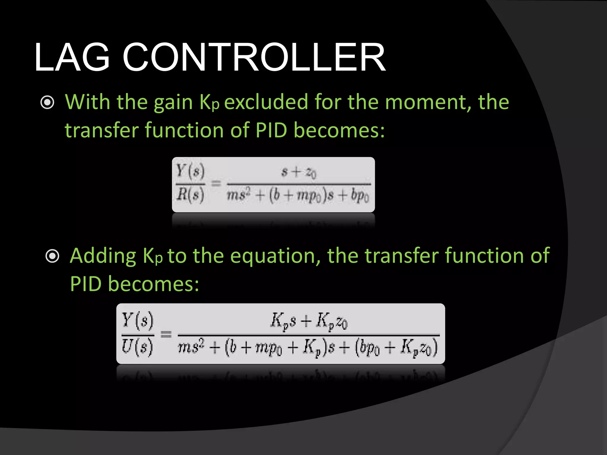
 With the gain Kp excluded for the moment, the
transfer function of PID becomes:
 Adding Kp to the equation, the transfer function of
PID becomes:
LEAD CONTROLLER
 The lead controller is basically added to
improve the transient response of the
system i.e. Ts and Tp mainly
 Not used here as it is not needed and the
desired parameters are already being
achieved
Cruise control simulation using matlab

Cruise control simulation using matlab

  • 1.
  • 2.
  • 3.
    CRUISE CONTROL  Cruisecontrol (speed control, auto-cruise or tempomat) is a system that automatically controls the speed of a motor vehicle. The system takes over the throttle of the car to maintain a steady speed as set by the driver.
  • 4.
  • 5.
    SYSTEM MODELLING  feedbackcontrol system  purpose is to maintain a constant vehicle speed despite external disturbances, such as changes in wind or road grade.  accomplished by i. measuring the vehicle speed ii. comparing it to the desired or reference speed iii. automatically adjusting the throttle according to a control law
  • 6.
    PHYSICAL SETUP: FBD bvu  Mass m  Control force u  Resistive forces bv  Vehicle velocity v  u = force generated at the road/tire interface  we will assume that : i. u can be controlled directly ii. the dynamics of the powertrain, tires, etc are 0 iii. bv, due to rolling resistance and wind drag varies linearly with the vehicle velocity, v, and act in the direction opposite the vehicle's motion
  • 7.
    FIRST ORDER EQUATION Weare considering a first order mass-damper system. Summing forces in the x-direction and applying Newton's 2nd law, we arrive at the following system equation: m(dv/dt)+bv=u Since v is the required output: y = v
  • 8.
    TRANSFER FUNCTION Taking theLaplace transform and assuming zero initial conditions, we find the transfer function of the cruise control system to be: P(s) = V(s)/U(s) = 1/(ms+b)
  • 9.
  • 10.
    PARAMETERS  m vehiclemass 1000 kg  b damping coefficient 50 N.s/m  r reference speed 10 m/s  Rise time < 5 s  Overshoot < 10%  Steady-state error < 2%
  • 11.
    BLOCK DIAGRAM C(s) P(s) Unitygain feedback controller C(s) = Kp + Ki/s + Kd.s
  • 12.
    PROPORTIONAL CONTROL  The root-locusplot shows the locations of all possible closed-loop poles when a single gain is varied from zero to infinity.  Only a proportional controller Kp will be considered to solve this problem. The closed-loop transfer function becomes: Y(s)/R(s) = Kp/(ms + ( b + Kp ) )
  • 13.
    PROPORTIONAL CONTROL  MATLAB commandsgrid  Used to display an acceptable region of the root-locus plot  Damping ratio (zeta) and the natural frequency (Wn) need to be determined
  • 14.
  • 15.
    PROPORTIONAL CONTROL  We canthen find a gain to place the closed- loop poles in the desired region by employing the rlocfind command  specific loop gain [Kp,poles]=rlocfind(P_cruise)  In between the dotted lines (zeta > 0.6) and outside the semi-ellipse (wn > 0.36)
  • 16.
    LAG CONTROLLER  Withthe gain Kp being the only functional gain and Ki and Kd being zero, the rise time and the overshoot criteria have been met  A steady-state error of more than 10% remains  To reduce the steady-state error, a lag controller is added to the system
  • 17.
    LAG CONTROLLER  Toreduce the steady-state error, a lag controller will be added to the system.  A pole and a zero, not too distant spacing- wise are introduced i.e:
  • 18.
    LAG CONTROLLER  Withthe gain Kp being the only functional gain and Ki and Kd being zero, the rise time and the overshoot criteria have been met  A steady-state error of more than 10% remains  To reduce the steady-state error, a lag controller is added to the system  the steady-state error will be reduced by a factor of zo/po
  • 19.
    LAG CONTROLLER  Withthe gain Kp excluded for the moment, the transfer function of PID becomes:  Adding Kp to the equation, the transfer function of PID becomes:
  • 20.
    LEAD CONTROLLER  Thelead controller is basically added to improve the transient response of the system i.e. Ts and Tp mainly  Not used here as it is not needed and the desired parameters are already being achieved

Editor's Notes

  • #15 The two dotted lines in an angle indicate the locations of constant damping ratio (zeta=0.6); the damping ratio is greater than 0.6 in between these lines and less than 0.6 outside the lines. The semi-ellipse indicates the locations of constant natural frequency (Wn=0.36); the natural frequency is greater than 0.36 outside the semi-ellipse, and smaller than 0.36 inside.