Comprehensive Study of Statistical Mechanics in Non-Equilibrium Phenomena
1.
Statistical mechanics ofnon-equilibrium
phenomena
M. K. Hassan
Professor, Department of Physics, Dhaka University
3.
Contents
1 Scaling, scale-invarianceand self-similarity page 1
1.1 Dimensions of physical quantity 4
1.1.1 Power-law monomial nature of dimensions 5
1.1.2 Significance of power-law monomial nature
of dimensional function 8
1.2 Buckingham π-theorem 11
1.2.1 Examples to illustrate significance of π-
theorem 14
1.3 Similarity 20
1.3.1 Illustrative Examples of similarity phe-
nomena 22
1.4 Self-similarity 25
1.4.1 Dynamic scaling and its link to π-theorem 28
1.4.2 Finite-size scaling and its link to π-theorem 29
1.5 Scale-invariance: Homogeneous function 31
1.5.1 Scale invariance: Generalized Homoge-
neous functions 33
1.5.2 Dimension functions are scale-invariant 35
1.6 Notes on power-law distribution 35
1.6.1 Examples of Power-law Distributions 38
1.7 Questions 38
1.8 Exercise 40
2 Stochastic process, random walk and diffusion 42
2.1 Stochastic Process 43
2.1.1 Essential Nomenclatures and Definitions: 45
2.2 Markov Process 47
2.2.1 Chapman-Kolmogorov Equation 48
4.
iv Contents
2.2.2 MarkovChains 49
2.2.3 Master Equation 49
2.3 Random walk (RW) problem 51
2.4 Master equation for RW problem 54
2.4.1 Diffusion equation for RW problem 56
2.4.2 Mean and root mean-square displacement 56
2.5 Diffusion and Fick’s Law 58
2.6 Brownian motion, diffusion and random walk 60
2.7 Solutions of diffusion equation 61
2.7.1 Exact solution 61
2.7.2 Scaling solution 62
2.7.3 Scaling Properties of the RW problem 65
2.8 Scale-free first return probability 67
2.8.1 Extensive numerical simulation to verify
power-law first return probability 72
2.9 Exercise 73
3 Stochastic theory of fragmentation 74
3.1 Master Equation for Binary Fragmentation Process 75
3.1.1 Properties of the daughter distribution
function 80
3.2 Ternery fragmentation 82
3.2.1 Fragmentation into an Arbitrary Number
of Particles 84
3.2.2 Definition of function c(x, t) and of its
various moments 84
3.3 Model I: Sum kernel: F(x, y) = (x + y)λ−1
86
3.4 Model II: Product kernel 91
3.5 Fragmentation of d dimensional objects 94
3.6 Solution to stochastic planar fragmentation 95
3.6.1 Multiscaling 98
3.7 Numerical simulation of the planar fragmentation 101
3.7.1 Algorithm of the planar fragmentation 101
3.8 Deterministic planar fragmentation 104
3.9 Exercise 105
4 Fractal and multifractal 109
4.1 Introduction 109
4.2 Euclidean geometry 111
4.3 Hausdorff-Besicovitch Dimension 114
4.4 Fractal 116
5.
Contents v
4.4.1 RecursiveCantor set (RCS) 117
4.4.2 Triadic Koch Curve 121
4.4.3 Sierpinski gasket and carpet 123
4.5 Similarity Dimension 126
4.6 Mass-length relation for fractal geometry 128
4.7 Truth about natural fractal 129
4.8 Dyadic Cantor set (DCS) 131
4.9 Kinetic DCS 133
4.10 Stochastic dyadic Cantor set 139
4.10.1 Data-collapse in kinetic DCS 145
4.11 Multifractality 147
4.12 Theory of Multifractality 149
4.12.1 Legendre transformation of τs(q): f(α)
spectrum 152
4.13 Cut and paste model on Sierpinski carpet 154
4.14 Stochastic Sierpinsky carpet 158
4.14.1 Discussions 164
4.15 Questions 166
5 Complex network theory 168
5.1 Introduction 168
5.2 What is network 170
5.3 Observables 172
5.3.1 Tree network and Complete graph 172
5.3.2 Degree k and degree distribution P(k) 172
5.3.3 Clustering co-efficient C 173
5.3.4 Mean geodesic (shortest) distance l 175
5.4 Random network: Erdos-Renyi model 176
5.5 Small-world network 178
5.5.1 Watts and Strogatz model 180
5.6 Scale-free complex network 181
5.6.1 The World Wide Web (WWW) 182
5.6.2 The Internet 182
5.6.3 Movie actor collaboration network 182
5.6.4 Scientific collaboration network 182
5.7 Barabasi-Albert model 183
5.8 Dynamic scaling and universility 190
5.9 Stochastic Planar Lattice 195
5.9.1 Kinetic square lattice 196
6.
vi Contents
5.9.2 Weightedplanar stochastic lattice by two
cracks (WPSL2) 198
5.9.3 Algorithm of the model 198
5.9.4 Topological properties of WPSL2 200
5.9.5 The role of group in the growth of BA
netwotk 202
5.9.6 Weighted planar stochastic lattice by a
single crack: WPSL1 206
5.9.7 Small-world properties of WPSL 209
5.10 Multi-multifractal properties of WPSL 211
5.10.1 WPSL2 211
5.10.2 WPSL1 212
6 Phase transition, critical phenomena and percola-
tion theory 216
6.1 The thermodynamic state functions: E, A, G, and H 216
6.2 The Legendre Tansformation 217
6.2.1 Thermodynamic Potentials 219
6.3 Response functions: Specific heat, compressibility
and susceptibility 220
6.3.1 Non-magnetic systems 220
6.3.2 Magnetic system 221
6.4 Stability and convexity relations and their geomet-
ric interpretation 222
6.5 Classification of phase transition 223
6.6 Critical Point exponent and universality 226
6.7 Widom Scaling 227
6.8 Percolation transition 230
6.9 Ovservable quantities in percolation 232
6.9.1 Spanning probability W(p) 232
6.9.2 Percolation probability P 233
6.9.3 Cluster size distribution function ns 234
6.9.4 Mean cluster size S 235
6.9.5 Connection to thermal phase transition 235
6.10 Exact solution in one dimension 236
6.10.1 Mean cluster size S 238
6.10.2 Correlation function g(r) and the correla-
tion length ξ 239
6.11 Percolation in the Bethe lattice: Exact solution 240
6.11.1 Properties of the Bethe lattice 240
7.
Contents vii
6.11.2 Percolationthreshold 241
6.11.3 Percolation strength P 242
6.11.4 Mean cluster size S 243
6.11.5 Correlation function g(r) 244
6.11.6 Cluster size distribution 244
6.12 Scaling theory 245
6.12.1 Cluster geometry 249
6.13 Finite-size scaling 252
6.14 Monte Carlo simulation 253
6.15 Hoshen-Kopelman algorithm 253
6.16 Newman-Ziff Algorithm 256
9.
1
Scaling, scale-invariance andself-similarity
Physics is all about observations and measurements of physical quanti-
ties with the desire to find some patterns in the data. These patterns
subsequently lead to finding principles of the phenomena under investi-
gation. The building blocks of physics are the physical quantities quan-
tify by numbers which are obtained by measurements. When we can
measure a physical quantity and express it in numbers only then we can
say we have gained some knowledge about that quantity; but when we
cannot express it in numbers then our knowledge about that quantity
can be described as meagre and unsatisfactory. Numbers to quantify
physical quantities are typically obtained by direct or indirect compari-
son with the corresponding units of measurements which are of two kind
such as fundamental and derivatives. The fundamental units of measure-
ments are defined arbitrarily in the form of certain standards, artificial
or natural, while the derivatives ones are obtained from the fundamental
units of measurements by virtue of the definitions which always indicates
some conceptual method or definition. For instance, the speed is the ra-
tio of the distance traversed in a given time interval to the magnitude of
that time interval and hence as unit of speed one can take the ratio of
the unit of length to the unit of time in the given system.
A set of fundamental units of measurement if sufficient for measuring
the properties of a class of phenomena under investigation then it is
called a system of units of measurement. Until recently, the centimeter-
gram-second system, abbreviated as CGS system, has been widely used
by scientists working in laboratories, dealing with small quantities where
one gram (g) is adopted as the unit of mass, one centimeter (cm) is
adopted as the unit of length, and one second (s) is adopted as the units
of time. A system of units of measurement consisting of two units such
as a unit for the measurement of length and a unit for the measurement
10.
2 Scaling, scale-invarianceand self-similarity
of time for example is sufficient for investigating the kinetic phenomena,
while a system of units consisting of only one length unit is sufficient for
measuring the geometric aspects of the object.
In addition to the CGS system, one often consider a system in which
1 km (105
cm) is used as the unit of length, 1 metric tonne (106
g) is
used as the unit of mass, and 1 hour (3600 s) is used as the unit of
time. These two systems of units have the following property in com-
mon: standard quantities of the same physical nature (mass, length, and
time) are used as the fundamental units. Consequently, we say that these
systems belong to the same class. To generalize, a set of systems of units
that differ only in the magnitude (but not in the physical nature) of the
fundamental units is called a class of systems of units. The system just
mentioned and the cgs system are members of the same class in which
standard lengths, masses and time are used as the fundamental units.
The corresponding units for an arbitrary system within the same class
are as follows: (i) unit of length = cm/L, (ii) unit of mass = g/M, and
(iii) unit of time = s/T, where L, M, T are the abstract positive numbers
that indicate the factors by which the fundamental units of length, mass
and time decreases in passing from the original system (in this case, the
cgs system) to another system in the same class. This class is called the
LMT class.
In particular, we find that one of the widely used the SI system belong
to the same LMT class, in which the unit of mass is taken to be 1
kg=1000 g, which is complete mass of the previously mentioned standard
of mass; the unit of length is taken to be 1 meter = 100 cm, which is
the complete length of the standard of length mentioned before; and the
unit of time is taken to be 1 second. Thus upon passage from the cgs
system to the SI system M = 0.001, L = 0.01, and T = 1. Often one
also uses systems of the FLT class, in which the fundamental units of
measurement have the form kgf/F, cm/L, and s/T . These are certainly
not the only possible choice of units of measurements rather the choice
of units of measurements depends on the scale of the physical quantity
under investigation. For instance in the study studying phenomena at
the atomic and molecular level it is useful to choose a unit of length
which is comparable to the size of an atom. We do this by using the
electron charge e as the unit of charge, and the electron mass me as the
unit of mass.
At the atomic level the forces are all electromagnetic, and therefore the
energies are always proportional to e2
4πǫ0
which has dimensions ML3
T −2
.
Another quantity that appears in quantum physics is h̄, the Plank’s
11.
Scaling, scale-invariance andself-similarity 3
constant divided by 2π which has dimensions ML2
T −1
. Dimensional
analysis then reveals that the atomic unit of length is
a0 =
h̄2
mee2
4πǫ0
. (1.1)
This is known as the Bohr radius or radius of smallest orbit for an elec-
tron circling around proton of the hydrogen atom. In astronomy we deal
with very large distances. It can be highly inconvenient to quote these
in meters and hence several other units are in use. For instance, the
astronomical unit (AU = 1.496 × 10¹¹
m) in which the average distance
between Earth and Sun is taken as the standard. The basic idea is that
the physical laws do not depend upon arbitrariness in the choice of the
basic units of measurement. Newton’s second law, F = ma, is true re-
gardless of whether we measure mass in kilograms, acceleration in meters
per second squared, and force in newtons, or whether we measure mass
in slugs, acceleration in feet per second squared, and force in pounds.
The measurement systems are of fundamental to physics as it allows us
to obtain the numerical number for quantifying different physical quan-
tities. However, the precise magnitude of the numerical value strictly
depends on the choice of the class of unit of measurements we use to
obtain it. Any investigation in physics ultimately comes down to deter-
mining certain quantity which may depend on various other physical
quantities that characterize the phenomena under consideration. The
problem therefore reduces to establishing relationship which can always
be represented in the form
f = f(a1, ..., an), (1.2)
where f is the quantity of primary interest which we will call governed
parameter and the quantities a1, a2, ..., an on which f depend on will
be called governing parameters. The governing parameters are usually
combined into one single term so that it bears the same physical dimen-
sion as the one for f. In this opening chapter we shall go over some
important aperitifs that we will need throughout this book. We will dis-
cuss the idea of dimension of physical quantity and how it differs from
dimensionless quantity. We will then rigorously prove that the dimen-
sional function of the physical quantity are always power-law monomial
in nature. The primary aim of this chapter is to establish the fact that
the scale-invariance, self-similarity or scaling as well as the mathemati-
cal definitions of the homogeneous function are all deeply rooted to the
power-law monomial nature of the dimensions of the physical quantity.
12.
4 Scaling, scale-invarianceand self-similarity
1.1 Dimensions of physical quantity
It can be said with certainty that each and everyone reading this book
have dealt with dimensional analysis is solving problems. Yet, do we
know enough to separate dimensionless quantity from a dimensional
quantity? It is absolutely essential to know a clearcut definition of the
dimension of physical quantity so that we can distinguish between the
two. Dimnension of a physical quantity is a function that determine the
number of times one needs to alter the numerical value of this quantity
while passing from one system of units of measurement to another sys-
tem within the same class. For instance, if the unit of length is decreased
by a factor L, the unit of mass is decreased by a factor of M and the unit
of time is decreased by a factor T then the unit of force is smaller by
a factor of MLT −2
than the original unit. Consequently, the numerical
values of all the forces are increased by a factor MLT −2
owing to the
definition of the principle of equivalence. Upon decreasing the unit of
mass by a factor M and the unit of length by a factor of L, we find that
the new unit of density is smaller by factor ML−3
than the original unit,
so that the numerical values of all the densities are increased by a factor
ML−3
. One can treat the other physical quantities of interest in the
similar fashion. On the other hand, quantities whose numerical values
remain identical in all systems of units within a given class are called
dimensionless and hence the dimension function is equal to unity for a
dimensionless quantity. We will find this definition extremely usefull not
only in this chapter but in the subsequent chapters as well.
Perhaps an example at this stage will provide a better understanding
about the dimensionless quantity than its mere definition. Consider that
the angular frequency ω of a pendulum of length l for small oscillations
is 9.8 cycle/sec. On the other hand using a simple dimensional analysis
or detailed solution reveals that the natural frequency of a pendulum
is
p
g/l where gis the acceleration due to gravity, which is 9 : 8 ms−2
on earth (in the SI system of units). To obtain the natural frequency of
the simple pendulum one usually needs to solve the differential equation
which results from applying Newton’s second law to the pendulum. It is
thus clear that the ratio
Π =
ω
p
g/l
, (1.3)
is a dimensionless quantity. Suppose that l = 1m and ω = 9.8cycles/sec
and hence Π =
√
9.8 in the SI system of units. Now let us change the
system of units so that the unit of mass is decreased by a factor of
13.
1.1 Dimensions ofphysical quantity 5
M = 1000, the unit of length is decreased by a factor of L = 100, and
the unit of time is decreased by a factor of T = 1. With this change, the
units of frequency will decrease by a factor of T −1
= 1 and the units
of acceleration by a factor of LT −2
= 100. Therefore, the numerical
value of l in the system of units of measurement will be l100 instead of
1 and that of g will be 980. However, the numerical value of Π is still
remain invariant under a change of units and hence it is a dimensionless
quantity.
1.1.1 Power-law monomial nature of dimensions
What is power monomial? A function a = φ(a, b, c, .., z) is called power-
law monomial if the different parameters a, b, ..., z combined together
into one term in the form of aα
bβ
...zγ
where the exact numerical value
of the exponents α, β, ...γ are fixed by the exact nature of the quantities
a, b, ..., z as well as the dimension of a itself. For instance in the case
of a = V the volume, its dimension function φ = φ(L, M, T) so that
[a] = Lα
Mβ
T γ
and hence the exponent α = 3 and the rest of the
exponents are zero. Indeed, there is no such instances where dimension
function can be expressed as Mexp[L] or sin M log T or L2
+ M−3
etc.
We see that all of the dimensions in the Table are power-law mono-
mials, of the form
[φ] = CLa
Mb
T c
...Iz
, (1.4)
where C is a constant and the exponents a, b, .., z assumes numbers en-
suring dimensional homogeneity. In fact, this is a general result which
can be rigorously proved. Indeed, the general proof of the theorem that
the dimension function of physical quantity always obey power mono-
mial law is highly instructive and it is elegant at the same time.
Proof: To prove this we consider a class of systems described by P,
Q, and R. By virtue of equivalence of systems within a given class, the
dimensions of any quantity a depend only on the quantities P, Q, and
R, i.e.,
[a] = f(P, Q, R). (1.5)
We now find it convenient to choose three systems of units denoted by
(0), (1), and (2). To be more precise, the systems of units (1) is obtain
from (0) by decreasing P, Q and R by a factor P1, Q1 and by a factor R1
respectively. On the other hand, the system of units (2) is similarly ob-
tained from (0) simply by decreasing the units of measurement P, Q, R
14.
6 Scaling, scale-invarianceand self-similarity
by a factor P2, Q2 and R2 respectively. Thus both the units of systems
(1) and (2) belong to the same class as the system (0) since all these three
systems differ from one another in the numerical value of their respec-
tive fundamental units of measurement. We can denote the dimension
of the physical quantity a in the systems (0) by [a] = f(P, Q, R) and
say that the numerical value of the quantity a measured in the system
(0) is equal to a. Now according to the definition of the dimensional
function, upon transition from the system (0) to the system (1) the
numerical value of the same quantity a increases by f(P1, Q1, R1) times
and hence the numerical value of the quantity a in the system (1) should
be equal to a1 = af(P1, Q1, R1). Similarly, upon transition from the (0)
to the system (2) the numerical of the quantity a is increased by a factor
f(P2, Q2, R2) and hence the numerical value of a when measured in the
system of unit of measurement (2) is a2 = af(P2, Q2, R2). Therefore,
applying the principle of equivalence we can write
a2
a1
=
f(P2, Q2, R2)
f(P1, Q1, R1)
, (1.6)
or
a2 = a1
f(P2, Q2, R2)
f(P1, Q1, R1)
, (1.7)
(0)
P, Q, R
1 1 1
P , Q , R
2 2 2
P , Q , R
2 1 2 1
Q /Q , R /R
(1)
(2)
/Q1
P
2
Figure 1.1 Schematic illustration of the transition among (0), (1) and
(2).
Hence it follows that the numerical values of the quantity a in the
systems (2) and (1) differ by f(P1, Q1, R1)/f(P2, Q2, R2). Now, let us
15.
1.1 Dimensions ofphysical quantity 7
consider that the system of unit of measurement (2) is obtained straight
from (1) instead of the system (0). In this case, the system (2) can be
obtained from the system (1) by decreasing the fundamental units by
factors of P2/P1, Q2/Q1 R2/R1 and as a result the the numerical value
of the corresponding quantity in question in system (2) would increase
by a factor f(P2/P1, Q2/Q1, R2/R1). That is, the numerical value of the
physical quantity a in (2) would be
a2 = a1f(P2/P1, Q2/Q1, R2/R1). (1.8)
Setting the above expression equal to Eq. (eq:1-2) we get the following
functional equation for the dimension function f:
f(P2, Q2, R2)
f(P1, Q1, R1)
= f(P2/P1, Q2/Q1, R2/R1). (1.9)
Perhaps an explicit simple example at this stage can provide better
clarity. Say, the length of a snack is measured in the MKS system and
found that its length is l0 = 5m which we refer as our original system
(0). Let another system of unit of measurement (1) is obtained from (0)
by decreasing the meter scale by a factor L1 = 100 (that is, cm). In doing
so the numerical value of the length of the snack is increased by factor
of f(L1) = 100 i.e., l1 = l0 × f(L1) = 500. Similarly, consider another
system of unit of measurement (2) is also obtained from (0) by decreasing
the meter scale by a factor of L2 = 1000 and hence the numerical value
of the length of the snack is increased by factor of f(L2) = 1000 i.e.,
l2 = l0 × f(L2) = 5000. Now, say the system (2) is obtained from
(1) instead of the system (0). It can be done by decreasing L1 by a
factor of (L2/L1) = 10 and hence the numerical value of l1 is increased
by a factor of 10 or l2 = l1 × f(L2/L1) = 5000. We thus see that
f(L2)/f(L1) = f(L2/L1).
To prove the theorem we differentiate both sides of Eq. (1.9) with
respect to P2 and then we set P2 = P1 = P, Q2 = Q1 = Q, R2 = R1 = R
to get
1
f(P, Q, R)
∂f(P, Q, R)
∂P
=
1
P
∂f(1, 1, 1)
∂P
≡
α
P
, (1.10)
where α ≡ ∂f(1,1,1)
∂P is a constant quantity, i.e. independent of P, Q, R.
Integrating the above equation we find
ln f(P, Q, R) = α ln P + C, (1.11)
where C is the integration constant that can be determined by setting
16.
8 Scaling, scale-invarianceand self-similarity
P = 1 to give C = ln f(1, Q, R) or C = ln f1(Q, R). f1 now is indepen-
dent of P. Substituting this into Eq. (1.11) we obtain
f(P, Q, R) = Pα
f1(Q, R). (1.12)
Putting it back in to Eq. (1.9) gives an equation for the function f1 of
the same form as we had for f except the that the new function f1 has
one argument fewer arguments than for f. That is,
f1(Q2, R2)
f1(Q1, R1)
= f1(Q2/Q1, R2/R1). (1.13)
Repeating the the same mathematical treatment as we did for f we get
1
f1(Q, R)
∂f1(Q, R)
∂Q
=
1
Q
∂f(1, 1)
∂Q
≡
β
Q
, (1.14)
Therefore,
f1 = Qβ
f2(R). (1.15)
Upon repeating once again we finally find
f = [a] = Pα
Qβ
Rγ
, (1.16)
The constant on the right hand side is equal to one since for P = Q =
R = 1 the system of units of measurement is unchanged and there is also
no change in the numerical value of the quantity a. Thus, the dimen-
sion of a physical quantity are always expressed by a power monomial.
The power monomial nature of the dimensional quantity is often called
dimensional homogeneity and it is really the key to dimensional analy-
sis. One can hardly exaggerate the importance of this law. For instance,
owing to this law one find that the laws of physics invariant under the
choice of units of measurement.
1.1.2 Significance of power-law monomial nature of
dimensional function
What are physical laws? They are usually relations between measured
or governed quantity and a set of governing parameters. For instance,
the Newton’s second law states that the acceleration a (the governed
parameter) experienced by an object depends on two governing param-
eters such as the mass m of the object and the net force F exerted on
it and hence can be written in the form
a = a(m, F). (1.17)
17.
1.1 Dimensions ofphysical quantity 9
That is, the physical laws can always be written in the form
Expression 1 = Expression 2. (1.18)
Then the power-law monomial nature of the dimensional function of
physical quantity implies that the governing parameters on the right
hand side must combine into one single term so that both sides of the
equation have the same dimensions and hence known as dimensional
analysis. Such identity could hold owing to the power-law monomial and
its homogeneity character of the dimensional functions. The following
examples might help us appreciate the importance and the significance
of the dimensional analysis.
Wingspan of an aircraft
We use the dimensional analysis to obtain the form of the dependence
of the lift for per unit wingspan on L, v and ρ where L is the width of
the wing, v is the velocity with which it is moving and ρ is air of density
through which the aircraft is moving.
Let us call the lift per unit wingspan Φ and write the following relation
Φ = kLα
vβ
ργ
, (1.19)
where k, α, β and γ are dimensionless constants. Using the dimension of
force MLT −2
we can immediately write the dimensional relation [w] =
MT −2
. Thus
MT −2
= Lα
Lβ
T −β
Mγ
L−3γ
. (1.20)
Applying the principle of equivalence we find γ = 1, β = 2 and solving
equation α + β − 3γ = 0 gives α = 1. We therefore can write
Φ = kLv2
ρ. (1.21)
This analysis suggests that we can define a dimensionless lift coefficient
η as
η =
F
1
2 Lρv2w
, (1.22)
where w is the width of the wingspan. Here the factor 1
2 is introduced
as matter of convention. Most aircraft wings have lift coefficient η in
the range 0.2 < η ≤ 0.6, depending on the design of the wing and its
orientation with respect to the motion of the aircraft.
18.
10 Scaling, scale-invarianceand self-similarity
Speed of traveling wave through a string:
We know that the wave velocity for a medium depends on the elastic
properties of the medium and on its inertia. Let us consider the simplest
one dimension case: a stretched string. Say, of the two remote ends, one
is attached to a far distance against a rigid wall and the other end is
at hand so that we can vary the tension on the string. It is clear that
the elastic character of the string is measured by the tension F and
the inertia character is measured by the mass density µ (mass per unit
length) of the string. If we flick our wrist once we can create a pulse that
will certainly propagate with some velocity. Detailed observation with
varying tension and changing string of different µ will convince that the
speed v of the pulse depends on both F and µ. Thus the dimension
velocity can be written in the following functional form
[v] = f(T, µ). (1.23)
Using the theorem that the dimension of physical quantity must follow
power monomial character we can immediately write
[v] = Fa
µb
. (1.24)
But, the dimension of velocity is LT −1
, of F is MLT −2
and of µ is
ML−1. Plugging these into the above equation gives
a + b = 0, and a − b = 1. (1.25)
Solving it we immediately find that a = 1/2 and b = −1/2 i.e.
v = C
s
F
µ
, (1.26)
where the constant C cannot be determined by dimensional analysis
alone. Nevertheless, one can use either theory or real life data to find
out that in this case it is C = 1.
On the other hand speed of traveling wave through a solid materiel
can also be obtained using the same technique. In this case the elastic
properties of the solid is determined by the Young’s modulus Y and its
inertia is determined by the density (mass per unit volume of the solid)
ρ. Using the technique we just used we find
v =
s
Y
ρ
. (1.27)
19.
1.2 Buckingham π-theorem11
Oscillation of a Star:
A star undergoes some mode of oscillation. How does the frequency ω
of oscillation depend upon the properties of the star? The first step is
the identification of the physically relevant governing variables on which
the success of the dimensional analysis depend on. Certainly, the density
ρ and the radius R are important; In addition to this the gravitational
constant G may play a role also the mass m but if we assume density is
constant then we have m = ρ(4πR3
/3) and hence the mass is a redun-
dant parameter. Thus, ω is the governed parameter with dimension T −1
,
and ρ, R and G are the governing parameters with dimensions ML−3
,
L and M−1
L3
T −2
respectively. Thus applying the fact that dimension
of all physical quantities follow power-law monomial we get
T −1
= [ρ]a
[R]b
[G]c
(1.28)
= Ma−c
L−3a + b + 3cT −2c
.
Equating the exponents on both sides gives three algebraic equations
and solving them immediately gives a = c = 1/2 and b = 0 so that
ω = C
p
Gρ, (1.29)
with C is a constant. We thus see that the frequency of oscillation is
proportional to the square root of the density and independent of the
radius R. Once again the determination of C requires real data or the-
ory. But either case a dimensional analysis helps focusing on the right
parameters with to right amount of importance.
1.2 Buckingham π-theorem
The name Pi comes from the mathematical notation Π are defined here,
for historical reason, to describe dimensionless variables obtained from
the power products of governing parameters denoted by Π1, Π2, Π3...
etc. If a physical process involves investigation of a certain dimensional
physical quantity (governed quantity) that depend on n number of other
dimensional variables then the Buckingham Pi theorem guide us in a sys-
tematic way to reduce a function of n variable problems into a function of
k dimensionless variable problems if each of the k dimensional variables
of the original n variables can be expressed in terms of the n − k dimen-
sionally independent variables. Now the question is: What is dimension-
ally independent variable? A set of dimensional variables, a1, a2, ..., ak of
the total n variables, is said to have independent dimensions if none of
20.
12 Scaling, scale-invarianceand self-similarity
the k variables have dimensions which can be represented as a product
of powers of the dimensions of the remaining variables. For instance,
density [ρ] = ML−3
, velocity [v] = LT −1
and force [F] = MLT −2
have
independent dimensions in the sense that none of these quantities can be
expressed in terms of the rest. In other words, there do not exist product
of powers of these quantities which is dimensionless. On the other hand
consider the case where force is replaced by pressure [P] = ML−1
T −2
.
In this case the dimension of pressure can be expressed in terms of the
dimension of that of velocity and density since [P] = [v2
][ρ] and hence
velocity and density have independent dimension but note the pressure.
Proof: The first step in modeling any physical phenomena are the
identification of the relevant variables, and then relating these variables
via known physical laws. For sufficiently simple phenomena, we can usu-
ally construct a quantitative relationship among the physical variables
from the first principles; however, for many complex phenomena such
an ab initio theory is often difficult, if not impossible. In these situ-
ations constructing a model in a systematic manners with minimum
input parameters that can help analyzing experimental results has been
a useful method, and one of the most powerful modeling method is
dimensional analysis. Most undergraduate have already encountered di-
mensional analysis during their course studies but without knowing its
full potential. Here we will use the dimensional analysis to capture tech-
niques for analyzing experimental or empirical data or to solve partial
differential equation which also help infer some insights about the solu-
tion. As we have already stated that the relationship found in physical
theories or experiments can always be represented in the form
a = f(a1, a2, ..., an), (1.30)
where the quantities a1, a2, ..., an are called the governing parameters.
Any investigation ultimately comes down to determining one or several
dependencies of the form Eq. (1.30). It is always possible to classify the
governing parameters a1, ..., an into two groups using the definition of de-
pendent and independent variables. Let the arguments ak+1, ..., an have
independent dimensions and the dimensions of the arguments a1, a2, ..., ak
can be expressed in terms of the dimensions of the governing indepen-
dent parameters ak+1, ..., an in the following way:
[a1] = [ak+1]α1
...[an]γ1
, (1.31)
[a2] = [ak+1]α2
...[an]γ2
,
... ... ...
21.
1.2 Buckingham π-theorem13
... ... ...
[ak] = [ak+1]αk
...[an]γk
.
The dimension of the governed parameter a must also be expressible in
terms of the dimensionally independent governing parameters a1, ..., ak
since a does not have independent dimension and hence we can write
[a] = [ak+1]α
...[an]γ
. (1.32)
Thus, there exist numbers α, β, and γ, such that Eq. (1.32) holds. We
can therefore a set of dimensionless governing parameters
Π1 =
a1
[ak+1]α1 ...[an]γ1
, (1.33)
Π2 =
a2
aα2
k+1...aγ2
n
,
... ... ...
Πk =
ak
[ak+1]αk ...[an]γk
,
and a dimensionless governed parameter
Π =
f(Π1([ak+1]α1
...[an]γ1
), ..., Πk([ak+1]αk
...[an]γk
, ak+1, ..., an)
[ak+1]α...[an]γ
.
(1.34)
The right hand side of this equation clearly reveals that the dimension-
less quantity Π is function of ak+1, ..., an, Π1, ..., Πk i.e.,
Π ≡ F(ak+1, ..., an, Π1, ..., Πk). (1.35)
The quantities Π, Π1, ..., Πk are obviously dimensionless, and hence
upon transition from one system of units to another inside the given
class their numerical values must remain unchanged. At the same time,
according to the above, one can pass to a system of units of measurement
such that any of the parameters of ak+1, ..., an, say for example, ak+1, is
changed by an arbitrary factor, and the remaining ones are unchanged.
Upon such a transition the first argument of F is changed arbitrarily,
and all the other arguments of the function remain unchanged as well as
its value Π. Hence, it follows δF
δak+1
= 0 and entirely analogously δF
δak+2
=
0, ... δF
δan
= 0. Therefore, the relation Eq. (1.35) is in fact represented by
a function of k arguments and proves it is independent of ak+1, ..., an
i.e.,
Π = Φ(Π1, ..., Πk), (1.36)
and the function f can be written in following special form
f(a1, ....., ak, ......., an) = aα
k+1.......aγ
nΦ((Π1, ...., Πk). (1.37)
22.
14 Scaling, scale-invarianceand self-similarity
Figure 1.2 A set of right triangles having the same lesser of the acute
angle θ
This constitutes the content of the central statement of dimensional anal-
ysis that has got far reaching consequence in understanding the scaling
theory. It is also known as the π-theorem that has been formulated and
proved for the first time E. Buckingham.
The importance and use of dimensional analysis and the Buckingham
π-theorem in particular in the description of the scaling or self-similarity
can hardly exaggerated. Theoretically, it is found that most physical
systems are governed either by partial differential or by partial integro-
differential equation and finding scaling or self-similarity will be subject
of intense and detailed consideration in the subsequent chapters. Never-
theless, here we give some instructive examples that will certainly help
grasping the essential ideas behind the π-theorem. In particular, the def-
inition of dimensionless quantity will play the central role in establishing
scaling or self-similarity.
1.2.1 Examples to illustrate significance of π-theorem
Area of a right triangle and Pythagorean theorem
Perhaps the simplest yet the most amusing example to demonstrate how
the idea of the π-theorem can be used to prove the Pythagorean theorem.
Consider a right tri-angle where three sides are of size a, b and c and,
for definiteness, the smaller of its acute angles θ. Assume that we are
23.
1.2 Buckingham π-theorem15
0
2
4
6
8
10
12
14
16
0 2 4 6 8 10
S
b
Figure 1.3 This figure shows how area S for one of the triangle of the
above figure (say the largest triangle) varies as the base b is changed.
to measure the area S of the triangle. The area S can be written in the
following form
S = S(a, b, c). (1.38)
However, the dimension of two governing parameters a and b can be
expressed in terms of c alone since we have
[a] ∼ [c] and [b] ∼ [c], (1.39)
and so is true for the governed parameter S as we can write the di-
mensional relation [S] ∼ [c2
]. We therefore can define two dimensionless
governing parameters
Π1 = sin θ = a/c and Π2 = cos θ = b/c, (1.40)
and the dimensionless governed parameter
Π =
S
c2
= c−2
S(cΠ1, cΠ2, c) ≡= F(c, Π1, Π2). (1.41)
Now it is possible to pass from one unit of measurement to another
system of unit of measurement within the same class and upon such
transition the arguments Π1 and Π2 of the function F as well as the
function itself remain unchanged. It implies that the function F is inde-
24.
16 Scaling, scale-invarianceand self-similarity
0
0.05
0.1
0.15
0.2
0.25
0 0.1 0.2 0.3 0.4 0.5 0.6 0.7 0.8 0.9 1
S/c
2
b/c
Figure 1.4 This shows that if we plot S/c2
vs b/c instead of S vs b
then all the three curves of figure (3) collapse on to a single master
curve. It implis that for a given numerical value of the ratio b/c
regardless of the size of the triangle corresponding S/c2
is the same
becuase triangle those satisfies these condition are similar and hence
the function φ(b/c) is unique.
pendent of c and hence we can write
Π = φ(Π1, Π2). (1.42)
However, Π1 and Π2 both depends on the dimensionless quantity θ and
hence we can write
S = c2
φ(θ), (1.43)
where the scaling function φ(θ) is universal in character.
In order to further capture the significance of Eq. (1.43) we re-write
it as
S
c2
∼ φ(θ). (1.44)
This result has far reaching consequences. For instance, consider that we
have a right triangle of any arbitrary sides a′
6= a, b′
6= b and c′
6= c but
have the same acute angle θ as before. This can be ensured by choosing
an arbitrary point on the hypotenuse of the previous triangle and drop a
perpendicular on the base b. Consider that the area of the new triangle
25.
1.2 Buckingham π-theorem17
is S′
yet we will have
S
c2
=
S′
(c′)2
, (1.45)
since the numerical value of the ratio of the area over the square of the
hypotenuse depends only on the angle θ. It implies that if we plot the
ratio of the area over the square of the hypotenuse as a function θ all
the data points should collapse onto single curve regardless of the size
of the hypotenuse and the respective areas of the right triangle. In fact,
the details calculation reveals that
φ(b/c) =
1
2
sin θ. (1.46)
Now the question is: What does this data collapse imply? It implies that
if two or more right triangles which have one of the acute angle identical
then such triangles are similar. We shall see later that whenever we will
find data collapse between two different systems of the same phenomenon
then it would mean that the corresponding systems or their underlying
mechanisms are similar. Similarly, if we find that data collected from
the whole system collapsed with similarly collected data from a suitably
chosen part of the whole system then we can conclude that part is similar
to the whole. On the other hand, if we have a set of data collected at
many different times for a kinetic system and find they all collapse onto
a single curve then we can say that the same system at different times
are similar. However, similarity in this case is found of the same system
at different times and hence we may coin it as temporal self-similarity.
Proof of the Pythagoras theorem: The area S of the original right
triangle is determined by the size of its hypotenuse c and the acute angle
θ since S = c2
φ(θ). Now, by drawing the altitude which is perpendicular
to the hypotenuse c we can divide the original triangle into two smaller
right triangles whose hypotenuses are a and b and say their respective
areas are S1 and S2. The two smaller right triangles will also have their
acute angle theta and hence we can easily show that
S1 = a2
φ(θ) and S2 = b2
φ(θ). (1.47)
On the other hand we have
S = S1 + S2, (1.48)
and it immediately lead to the conclusion that c2
= a2
+b2
which is just
the Pythagorean theorem.
26.
18 Scaling, scale-invarianceand self-similarity
Figure 1.5 A schematic diagram showing the experiments of Bose,
Rauert and Bose. The time τ requered to fill a vessel of volume Q
and the pressure drop between the ends of the pipe P were measured
for the steady flow of various fluids through the pipe.
Bose-Rauert-Bose experiment
In 1909-1911 the physical chemists E. Bose, D. Rauert, and M. Bose
performed a series of experimental investigations based on the scheme
as described by the Fig. . The experiment consist in measuring the nec-
essary time τ to fill a container of given volume V and the pressure
drop P at the ends of a pipe for steady flow of various fluids e.g. water,
chloroform, mercury, ethyl alcohol e.t.c. through the pipe. The experi-
mental results are represented in the form of a series of curves for the
presurre drop as a function of the filling time τ for various fluids, like
those shown in Fig... The work was subsequently noted by von Karman
who performed a dimensional analysis to give a better interpretation of
the experimental results.
Von Karman’s arguments can be presented as follows. The pressure
drop P at the ends of the tubes must depends on the parameters such as
the filling time τ, the volume V of the container, the viscosity coefficient
µ and the density ρ of the fluid used. So these are the four governing
parameters which are expected to govern the phenomena in question
and hence n = 4. The dimensions of the parameters in the MLT class
can be expressed by the following relations:
[P] =
M
LT 2
, [τ] = T, [V ] = L3
, [µ] =
M
LT
, [ρ] =
M
L3
. (1.49)
27.
1.2 Buckingham π-theorem19
Figure 1.6 The experimental results of Bose, Rauert and Bose in their
original form: ◦ for water, • for chloroform; + for bromoform; △ for
mercury. The curves are different for the different fluids.
Figure 1.7 The experimental results of E. Bose, D. Rauert, and M.
Bose. as represented vy von Karan in 1911, who used dimensional
analysis. Point to note is that the experimental points for different
fluids lie on a single curve.
28.
20 Scaling, scale-invarianceand self-similarity
It is easy to see that the first three governing parameters τ, µ and V have
independent dimensions, while the dimensions of the fourth governing
parameter, ρ, are expressed in terms of the first three: [ρ] = [µ][τ][V ]2/3
.
Thus we have k = 3, so that n − k = 1, and dimensional analysis gives
Π = Φ(Π1), Π =
P
µτ−1
, Π1 =
ρ
µτV −2/3
. (1.50)
Consequently, according to the above equation, had we plot in the coor-
dinates Π and Π1, all the experimental points should fall on to a single
curve as is confirmed by the Fig.
1.3 Similarity
In most cases, before a large and expensive structure or object such as
a ship or aeroplane is built, efforts are always devoted to the testing
on model system instead of working directly with the real system. The
results of testing on model system are then used to infer the various
physical characteristics of the real object or structure under the future
working conditions. In order to successful modeling, it is necessary that
we know how to relate the results of testing on models to the actual
manufactured product. Needless to mention that if such connections are
not known or cannot be made then modeling is simply a useless pursuit.
For the purpose of rational modeling, the concept and the importance
of the similarity phenomena can hardly be over emphasized. Indeed, the
physically similar phenomena is the key to successful modeling.
The concept of physical similarity is a natural generalization of the
concept of similarity in geometry. For instance, two triangles are similar
if they differ only in the numerical values of the dimensional param-
eters, i.e. the lengths of the sides, while the dimensionless parameters,
the angles at the vertices are identical for the two triangles. Analogously,
physical phenomena are called similar if they differ only in their numer-
ical values of the dimensional governing parameters; the values of the
corresponding dimensionless parameters Π1, ..., Πm are being identical.
In connection with this definition of similar phenomena, the dimension-
less quantities are called similarity parameters.
Let us consider two similar phenomena, one of which will be called
the prototype and the other the model; it should be understood that
this terminology is just a convention. For both phenomena there is some
29.
1.3 Similarity 21
relationof the form
a = f(a1, a2, a3, b1, b2), (1.51)
where the function f is the same in both cases by the definition of
similar phenomena, but the numerical values of the governing parameters
a1, a2, a3, b1, b2 are different. Thus for prototype we have
ap = f(a
(p)
1 , a
(p)
2 , a
(p)
3 , b
(p)
1 , b
(p)
2 ), (1.52)
and for for model system we have
am = f(a
(m)
1 , a
(m)
2 , a
(m)
3 , b
(m)
1 , b
(m)
2 ), (1.53)
where the index p denotes quantities related to the prototype and the
index m denotes quantities related to the model. Consider that b1 and
b2 are dependent variables so that they can be expressed in terms of
a1, a1 and a3 in both model and prototype systems. Using dimensional
analysis we find for both phenomena
Π(p)
= Φ(Π
(p)
1 , Π
(p)
2 ), (1.54)
and
Π(m)
= Φ(Π
(m)
1 , Π
(m)
2 ), (1.55)
where the function Φ must be the same for the model and the prototype.
By the definition of similar phenomena the dimensionless quantities must
be identical in both the cases such as in the proto-type and in the model
i.e.,
Π
(m)
1 = Π
(p)
1 , Π
(m)
2 = Π
(p)
2 . (1.56)
It also follows that the governed dimensionless parameter satisfies
Π(m)
= Π(p)
. (1.57)
Returning to dimensional variables, we get from the above equation
ap = am
a
(p)
1
a
(m)
1
p a
(p)
2
a
(m)
2
q a
(p)
3
a
(m)
3
r
, (1.58)
which is a simple rule for recalculating the results of measurements on
the similar model for the prototype, for which direct measurement may
be difficult to carry out for one reason or another.
The conditions for similarity of the model to the prototype-equality
of the similarity parameters Π1, Π2 for both phenomena show that it is
30.
22 Scaling, scale-invarianceand self-similarity
necessary to choose the governing parameters b
(m)
1 , b
(m)
2 , of the model so
as to guarantee the similarity of the model to the prototype:
b
(m)
1 = b
(p)
1
a
(m)
1
a
(p)
1
α1
a
(m)
2
a
(p)
2
β1
a
(m)
3
a
(p)
3
γ1
, (1.59)
and
b
(m)
2 = b
(p)
1
a
(m)
1
a
(p)
1
α2
a
(m)
2
a
(p)
2
β2
a
(m)
3
a
(p)
3
γ2
, (1.60)
whereas the model parameters a
(m)
1 , a
(m)
2 , a
(m)
3 can be chosen arbitrar-
ily. The simple definitions and statements presented above describe the
entire content of the theory of similarity: we emphasize that there is
nothing more to this. We will now give a few examples to help us cap-
ture the idea.
1.3.1 Illustrative Examples of similarity phenomena
(i) The steady motion of a body in a large vessel filled with
fluid:
To do this we consider the following assumptions:
(a) The velocity of the body is assumed to be small relative to the
velocity of sound, so that the fluid can be treated as incompressible and
hence of constant density.
(b) The direction of the velocity vector assumed to be identical for both
model and proto-type which is the case if the model and the proto-type
are geometrically similar.
In this problem, the dimensional governing parameters of the motion
are the characteristic length scale of the body such as the maximum
cross-sectional diameter D, the magnitude v of the body’s velocity, the
density ρ of the fluid, and finally its viscosity µ. The dimensions of the
governing parameters are
[D] = L, [v] = LT −1
, [ρ] = ML−3
, [µ] = ML−1
T −1
. (1.61)
31.
1.3 Similarity 23
Asimple dimensional analysis will immediately reveal that n = 4 and
m = 1 so that there is only one governing dimensionless parameter
Π1 =
ρvD
µ
. (1.62)
As proposed by A Sommerfeld, this parameter is called the Reynolds
number in honor of the English scientist Osborne Reynold who was
one of the first to apply the ideas of similarity to hydrodynamics with
remarkable success. The dimensionless governed parameter or the drag
force on the body can be naturally defined as
Π =
F
1
2 v2S
, (1.63)
where F is the drag force on the body, S ∼ D2
is the cross-sectional
area of the body, and the factor 1/2 in the denominator is introduced
by tradition.
The function Π(Re) for the flow past a sphere is shown in the fol-
lowing figure. To a very high accuracy, the data from a large number
of experiments for very many different size of the body lie on a sin-
gle curve. This curve appears to be very complicated: regions in which
Π(Re) varies smoothly alternate with sharp decrease and increases, and
there are regions where Π is almost independent of Re. This all indicates
that the flow regimes very with reynolds number.
The motion of a model is usually implanted in the same fluid as that
in which the proto type moves. The similarity condition that the di-
mensionless parameter Π1 be the same for the model and the proto type
motions indicates that in this case, the product vD must be identical for
model and for the prototype; from this we see that the velocity at which
a dynamically similar model moves is inversely proportional to the size
of the model compared with that of prototype. From this, it follows that
the drag forces are identical for the model and the prototype, so that
the scaling coefficients for the drag force is equal to unity in this case.
(ii) The Motion of a Streamlined Surface Ship at High Speeds:
Here, we shall discussed the idealized case where the contribution from
viscous drag can, to a rough approximation, be assumed to be small for
a stremlined ship; the main contribution to the drag ona ship in rapid
32.
24 Scaling, scale-invarianceand self-similarity
motion is that due to the surface waves created by the ship. The govern-
ing parameters in this case at hand will be as follows: a characteristic
length for the ship, l, the gravitational acceleration g, the density of the
fluid ρ, and the speed of the ship v. the parameter g is essential since the
gravitational force is one of the factors that controls the waves created
by the ship. The governing parameters have the following dimensions in
the LMT class:
[l] = L, [v] = LT −1
, [ρ] = ML−3
, [g] = LT −2
, (1.64)
so that n = 4, k = 3, and m = 1 which implies that there is only one
dimensionless governing parameter
Π1 =
v
l1/2g1/2
. (1.65)
This parameter is called the Froude number which is named after famous
English engineer and ship builder Wm. Froude.
Furthermore, the dimension of the drag force F in the same class
LMT is [F] = [ρ][g][l]3
so that dimensionless governed drag force is
Π =
F
l1/2g1/2
. (1.66)
Thus, since the parameter g can hardly be varied, the law for scaling
the drag forces from the model up to the prototype in the same fluid is
of the form
F(p)
= F(m)
l(p)
l(m)
3
, (1.67)
so that the drag force is proportional to the cube of the modeling scale.
Relation for the dimensionless governing parameter indicates that in
order to ensure dynamical similarity, the ratio of the model velocity to
the prototype velocity must be proportional to the square root of the
modeling scale:
v(m)
= v(p)
l(m)
l(p)
1/2
. (1.68)
If one does not neglect the role of the viscosity, a second dynamical
parameter appears - the Reynolds number Re, which is equal to ρvl/µ.
Modeling in which both similarity parameters - the Froude number and
Reynolds number - are taken into account turns out to be impossible in
the same fluid. indeed, to do this , the products vl (see example (i) above)
and v2
/l would have to be identical for both model and the prototype;
this is only possible when modeling to full scale, which makes no sense.
33.
1.4 Self-similarity 25
Thisis precisely why, for illustration, we have restricted ourselves to the
case where viscous drag is small compared with the wave drag.
1.4 Self-similarity
The notion of self-similarity will be an underlying theme for the rest
of the book. In a way the word self-similarity needs no explanation.
Perhaps the best way to perceive the meaning of self-similarity is to
consider an example and at this stage there is no better example than
a cauliflower. The cauliflower head contains branches or parts, which
when removed and compared with the whole found to be very much
the same except it is scaled down. These isolated branches can again
be decomposed into smaller parts, which again look very similar to the
whole as well as of the branches. Such self-similarity can easily be car-
ried through for about three to four stages. After that the structures are
too small to go for further dissection. Of course, from the mathematical
point of view the property of self-similarity may be continued through
an infinite stages though in real world such property sustain only a few
stages. Self-similarity can also be found on smaller scales. For instance,
snowflakes often display self-similar branching patterns and aggregating
colloidal particles have growth patterns that are statistically self-similar.
Self-similarity, in fact, is so widespread in nature that they are exceed-
ingly easy to find. Consequently, the main ideas of self-similarity are not
difficult to grasp. Hopefully, when we are done with this chapter, we will
have the basic understanding of self-similar phenomena and when are
done with the whole book we will be able to appreciate the fact that
self-similar phenomena are ubiquitous in nature as it is virtually every-
where we look. In our endeavour we need to spend just a few minutes
laying the foundation for that knowledge. We begin our exploration with
three more examples of self-similarity.
Firstly, think of a lone leafless tree standing against a gray winter
sky as the background. Needless to mention that branching patterns
are quite familiar to us. There is a single trunk that rises to a region
from where major branches split off. If we follow any one of these major
branches, we see that they also split into smaller branches, which split
into even smaller branches, and so on. A unit pattern (in this case one
length splitting into two or more thinner branches) is repeated on ever-
smaller size scales until we reach the tree-top. Having this picture in
mind, we can state a simple generic definition: the fundamental principle
34.
26 Scaling, scale-invarianceand self-similarity
of a self-similar structure is the repetition of a unit pattern on different
size scales. Note that the delicate veins of leaves also have self-similar
branching patterns, as do virtually all root systems. A tree is therefore
the epitome of self-similarity.
Secondly, the decimal number system which is probably the oldest and
most useful construction that used the idea of self-similarity. However,
we use it so much in our daily life that we hardly had time to appreciate
its self-similar properties. Let us look at the meter stick, which has marks
for decimeters (ten of it make a meter), centimeters (ten of it makes a
decimeter and a thousand make a meter), milimeters (ten of it makes
a centimeter). In a sense a decimeter together with its marks look like
a meter with its marks, however, scaled down by a factor of 10. This is
not an accident. It is in strict correspondence with the decimal system.
When we say 248 mm, for example, we mean 2 decimeters, 4 centimeters,
and 8 millimeters. In other words, the position of the figures determines
their place value, exactly as in the decimal number system. One meter
has a thousand millimeters to it and when we have to locate position
248 only a fool would start counting from left to right from 1 to 248.
rather we would go to the 2 decimeter tick mark, from there to the four
centimeter tick mark, and from there to the 8 millimeter tick mark. Most
of us take this elegant procedure for granted. But somebody who has
to convert miles, yards, and inches can really appreciate the beauty of
this system. Actually finding a position on the meter stick correspond
to walk on the branches of a tree, the decimal number. the structure of
the tree expresses the self-similarity of the decimal system very strongly.
Thirdly, distant mountain range which is an example of statistical
self-similarity as we find hierarchy of peak/valley morphologies on size
scales ranging from kilometers to centimeters. This is in sharp contrast
to the above mentioned decimal system. Such self-similarity is found true
in almost all the surfaces we encounter since in majority of them have
hierarchy of self-similar structure over at least some range of size scales.
Consider the vast craters-within-craters surface of the Moon displaying
self-similar divots that range in diameter from kilometers to millimeters.
Erosion processes in desert regions yield a wealth of self-similar surfaces,
and areas of snow and ice, from the vast continent of Antarctica to
the piles of snow next to our driveways, have self-similar structures.
There are examples of statistical self-similarity in the plant kingdom
too. Ferns and cedar boughs have pleasing multi-leveled designs that
are strongly self-similar. The overall shape of the fronds or boughs is
roughly that of a broad sword with sharp tip and a stem running along
35.
1.4 Self-similarity 27
itsmidline. However, a closer look reveals that it is actually composed
of many small swords oriented at right angles to the main stem. These
second-level swords, in turn, are divided into third-level swords lying
roughly perpendicular to the second-level stems. Perhaps many of us
had been looking on countless occasion at many seeming self-similar
structure without really appreciating their true self-similar design.
One may even find self-similarity in social systems if one thinks about
how our governments, judicial systems, law enforcement agencies or var-
ious economic systems work. It is fairly easy to see that they have almost
discrete hierarchical arrangements with federal, state, local upto family
levels. Basically a similar type of activity is occurring at the different
scales and so we find a familiar design in a new context. The main princi-
ple of self-similarity - same thing on different scales - can be found in fact
in countless examples from the social sectors. The Internet has grown
according to the laws of self-similarity and its complex multi-scaled net-
working in actually result from the repeatation of simple law. Multi-
scaled networking is reminiscent of the self-similar networking structure
in the brain of living systems. Likewise the growth patterns and inter-
connectedness of cities exhibit similar phenomena on different scales, the
hallmark of self-similarity. Well, we could go on with further examples
of self-similarity such as lightning bolts, designs on shells, aggregation
of bacteria or metal ions, surfaces of cancer cells, crystallization pat-
terns in agate, scores of scaling laws in biology, quantum particle paths,
gamma-ray burst fluctuations, species distributions or abundances, drop
formation, renormalization in quantum electrodynamics, and so on. We
will have many opportunities in the chapter to come to add more exam-
ples because it can said beyond any reasonable doubt that nature adores
self-similarity.
In physics we often investigate physical problem which we do not see
by our naked eye and hence cannot appreciate straight away if the sys-
tem possess self-similarity. However, we attempt to solve them through
modeling which are often governed or described by kinetic or rate equa-
tion approach. Mathematician and physicists often look for scaling or
self-similar solution to their respective equations which is the solution
in the long time limit. In this limit, the solution usually assumes simpler
and universal form. An equation is considered to assume self-similar or
scaling solution if its solution has either power-law form or have the
dynamic scaling form which are discussed below.
36.
28 Scaling, scale-invarianceand self-similarity
1.4.1 Dynamic scaling and its link to π-theorem
A function f(x, t) is said to obey dynamic scaling if one of the variable
t strictly denotes time (time developing phenomena) and if it satisfies
f(x, t) ∼ tτ
φ(x/tz
), (1.69)
where exponents θ and z are fixed by the dimensional relations [tθ
] = [f]
and [tz
] = [x] respectively, while φ(ξ) is known as the scaling function.
Sometimes it is also written in the following form
f(x, t) ∼ xω
φ(x/tz
). (1.70)
Both the form came into being as hypothesis since its deep connection
to Buckingham π-theorem has never been appreciated. Indeed, Bucking-
ham π-theorem can provide a systematic processing procedure to obtain
the dynamic scaling form and at the same time appreciate the fact that
the second form is not mathematically sound. An interesting aspect of
the structure of the dynamic scaling form given by Eq. (1.69) is that the
distribution function f(x, t) at various moments of time can be obtained
from one another by a similarity transformation
x −→ λz
x, t −→ λt, f −→ λθ
f, (1.71)
revealing the self-similar nature of the function f(x, t).
To derive it one has to know first that one of the two governing pa-
rameters can be assumed to be independent. Let us assume that t is
chosen to be an independent parameter and hence x can be expressed
in terms of t
x ∼ tz
. (1.72)
It implies that we can choose tz
as unit of measurement or yard-stick
and quantify x in terms of dimensionless quantity ξ = x/tz
. Here, the
quantity ξ is a number that tells how many tz
we need to measure x.
If t is independent quantity then we can also express f in units of tτ
to obtain yet another dimensionless quantity φ = f(x, t)/tτ
where the
exponent θ is fixed by the dimensional requirement [f] = [tθ
]. Since
φ is a dimensionless quantity its numerical value can only depend on
dimensionless quantity ξ not on depend on a dimensional quantity t. This
is reminiscent of that fact that the numerical value of S/c2
is independent
of the size of the hypotenuse c for fixed value of the lesser angle θ. We
can then immediately obtain the scaling form given by Eq. (1.69). On
the other hand, had we choose x to be independent parameter instead of
37.
1.4 Self-similarity 29
tthen following the same argument we would have the following scaling
form
f(x, t) ∼ xω
φ(t/xν
), (1.73)
where ν = 1/z. Note that if we express f in unit of x then t should also
be expressed in unit of x.
There are many phenomena which physicist often investigate are not
static rather evolve probabilistically with time. In such cases too one
often is interested to see if certain distribution function of the systems at
different times are similar. In fact, we use the very definition of similarity
but not two different systems but of the same system at various moments
of time. Emergence of dynamic scaling is in fact deeply rooted to the
Buckingham’s π-theorem. Note that one can derive the dynamic scaling
form if we find that one of the two variables of the function f(x, t), say
t, has independent dimension and the dimension of the other variable
x can be expressed in terms of t alone i.e. [x] ∼ [tz
]. This means that
the function f can also be expressed in terms of the dimension of t and
satisfy the dimensional relation [f] = [tθ
]. Following the steps of the
Buckingham’s π-theorem can immediately led to the dynamic scaling
form. Existence of dynamic scaling also means existence temporal self-
similarity since it implies that the dimensionless quantities at different
time must be identical. Indeed, one way of verifying the dynamic scaling
is to plot dimensionless variables f/tθ
as a function of x/tz
of the data
extracted at various different time. Then if all the plots collapse onto a
single universal curve then it is said that the systems at different time
are similar and it obeys dynamic scaling. Essentially such systems can
be termed as temporal self-similarity since the the same system is similar
at different times.
1.4.2 Finite-size scaling and its link to π-theorem
There exists yet another scaling hypothesis, known as the finite-size scal-
ing (FSS), that has been extensively used as a very powerful tool for es-
timating finite size effects specially in the second order phase transition
near the critical temperature T . The various response functions, typi-
cally the second derivative of the free-energy F, in second order phase
transition diverges. Such transitions are classified by a set of critical ex-
ponents which characterize the critical point. The best known example
of second order phase transition is the paramagnetic to ferromagnetic
38.
30 Scaling, scale-invarianceand self-similarity
transtion where
Magnetization M ∼ (T − Tc)β
Susceptibility χM ∼ (T − Tc)−γ
Heatcapacity CV ∼ (T − Tc)−α
Correlation length ξ ∼ (T − Tc)−ν
. (1.74)
These relations are only true in the thermodynamic limit in the sense
that the system size is infinite. However, we can work in simulation
and experiment only with finite size Ld
where correlation lenght ξ ∼ L.
Finite-size scaling thus provides a means of extrapolating various results
for infinite systems.
According to finite=size scaling (FSS) hypothesis, a function f(ǫ, L)
with ǫ = (T − Tc) is said to obey finite size scaling if it can be expressed
as
f(ǫ, L) ∼ L−ω/ν
φ((T − Tc)L1/ν
). (1.75)
However, using the Buckingham π-theorem we not only obtain the cor-
rect scaling form but we also gain a deeper insight into the problem as
it provides a systematic processing procedure. For instance, as we know
that the correlation length ξ in the limit L → ∞ diverges like ξ ∼ ǫν
near the critical point and it bear the dimension of length. We therefore
can either choose L as an independent parameter and measure ξ vis-a-
vis T − Tc in unit of L or we can measure L in unit of T − Tc assuming
it as an independent parameter. Choosing the later case we can define
a dimensionless quantiy
π =
L
ξ
= L(T − Tc)ν
, (1.76)
and the corresponding dimensionless governed parameter is
Π =
f(ǫ, L
ξω
= φ(π). (1.77)
Following the argument of the π-theorem we can immediately write that
f(ǫ, L) ∼ (T − Tc)−νω
φ(L(T − Tc)ν
). (1.78)
On the other hand had we chosen L as an independent parameter then
the similar treatment would yield
f(ǫ, L) ∼ Lθ
φ({L(T − Tc)ν
}−1
). (1.79)
39.
1.5 Scale-invariance: Homogeneousfunction 31
Till to-date neither of the two scaling forms obtained folliwing π-
theorem are in use in their strict form. Instead, what is done tradionally
are as follows. The important point is that if π = L/ξ is dimensionless
then so is
π1/ν
= (L/ξ)1/ν
= (T − Tc)L1/ν
. (1.80)
It also means that we can choose L as independent parameter and ex-
press (T −Tc) in unit of L−1/ν
to make the dimensionless quanity coincide
with π1/ν
. Then f too can be expressed in unit of Lθ
which according
to the prescription of π-theorem we have the following FSS scaling form
f(ǫ, L) ∼ Lθ
φ((T − Tc)L1/ν
), (1.81)
which is the same as the traditional scaling form given by Eq. (1.75) if
we find θ negative and it is related to the exponent ν via θ = −ω/ν.
A quantitative way of interpreting how the experimental data ex-
hibits finite-size scaling is done by invoking the idea of data-collapse
method - an idea that goes back to the original observation of Rush-
brooke. That is, the values of f(ǫ, L) for different system size L can be
made to collapse on a single curve if fLω/ν
is plotted against ǫL1/ν
. It
implies that systems of different sizes are all similar that also include
system where l → ∞. The method of data-collapse therefore comes as
a powerful means of establishing scaling. It is extensively used to an-
alyze and extract exponents especially from numerical simulations. We
shall elucidate it further in the chapter on phase transition, percolation
theory and critical phenomena.
1.5 Scale-invariance: Homogeneous function
A function is called scale-invariant or scale-free if it retains its form
keeping all its characteristic features intact even if we change the mea-
surement unit (scale). Mathematically, a function f(r) is called scale-
invariant or scale-free if it satisfies
f(λr) = g(λ)f(r) ∀ λ, (1.82)
where g(λ) is yet unspecified function. That is, one is interested in the
shape of f(λr) for some scale factor λ which can be taken to be a length
or size rescaling. For instance dimensional functions of physical quantity
are always scale-free since they obey power monomial law. In fact, it
40.
32 Scaling, scale-invarianceand self-similarity
can be rigorously proved that the function that satisfy Eq. (1.82) should
always have power-law form f(r) ∼ r−α
.
Proof: Starting from Eq. (1.82), let us first set x = 1 to obtain f(λ) =
g(λ)f(1). Thus g(λ) = f(λ)/f(1) and Eq. (1.82) can be written as
f(λx) =
f(λ)f(x)
f(1)
. (1.83)
The above equation is supposed to be true for any λ, we can therefore
differentiate both sides with respect to λ to yield
xf′
(λx) =
f′
(λ)f(x)
f(1)
, (1.84)
where f′
indicates the derivative of f with respect to its argument. Now
we set λ = 1 and get
xf′
(x) =
f′
(1)f(x)
f(1)
.n (1.85)
This is a first-order ordinary differential equation which has a solution
f(x) = f(1)x−α
, (1.86)
where α = −f(1)/f′
(1). It clearly proves that the power-law type is the
only solution that can satisfy Eq. (1.82).
In fact, it can also be proved rigorously that g(λ) too have the power-
law solution.
Proof: Suppose we make two changes of scale, first by a factor of µ
and then by by a factor of λ. The homogeneity condition of the function
f(r) implies
f λ(µr)
= g(λ)f(µr) = g(λ)g(µ)f(r). (1.87)
A similar result can also be obtained by a single change of scale as follows
f (λµ)r
= g(λµ)f(r). (1.88)
By applying the principle of equivalence of the above two equations we
obtain
g(λµ) = g(λ)g(µ). (1.89)
Now any continuous function that satisfies the above functional equation
must be either identically zero or else will have a simple power-law form
with respect to its argument. To prove this we take the derivative with
respect to µ, we find
∂
∂µ
g(λµ) = λg′
(λµ) = g(λ)g′
(µ), (1.90)
41.
1.5 Scale-invariance: Homogeneousfunction 33
where prime indicates derivative with respect to the argument of the
corresponding function. We now set µ = 1 and g′
(1) = p then we can
immediately write
1
g(λ)
g′
(λ) =
p
λ
. (1.91)
Integrating it we find
ln[g(λ)] = p ln[λ] + c, (1.92)
or
g(λ) = ec
λp
. (1.93)
Now from the above equation we have g′
(λ) = pec
λp−1
and the definition
g′
(1) = p implies that the integration constant c has the value zero. Thus
g(λ) ∼ λp
, (1.94)
and it makes the proof complete.
The power-law type distributions f(x) ∼ x−α
are regarded as scale-
free because f(λx)/f(x) depends only on λ not on x and hence their
distribution requires no characteristic or typical scale. The idea is that
if the unit of measurement of x is increased (decreased) by a factor of λ
then the numerical value of f is decreased (increased) by a factor of g(λ)
but the overall shape of the function remains invariant. It is called scale-
free also because it ensures self-similarity in the sense that the function
looks the same whatever scale we look at it. One immediate consequence
of the scale-invariant function f(r) is that if we know its value at one
point say at r = r0, and we know the functional form of g(λ), then the
function f(r) is known everywhere. This follows because any value of r
can always be written in the form r = λr0, and
f(λr0) = g(λ)f(r0). (1.95)
The above equation says that the value f(r) at any point is related to
the value of f(r0) at a reference point r = r0 by a simple change of scale.
Of course, this change of scale is, in general, not linear.
1.5.1 Scale invariance: Generalized Homogeneous
functions
We shall see latter in the static scaling hypothesis where we shall use the
fact that the thermodynamic potentials are homogeneous of the form A
function f(x, y) of two independent variables x and y is said to be a
42.
34 Scaling, scale-invarianceand self-similarity
generalized homogeneous function if, for all values of the parameter λ
f(x, y) satisfies
f(λa
x, λb
y) = λf(x, y), (1.96)
where a and b are arbitrary numbers. In analogy with the homogeneous
function why does not one define the generalized homogeneous function
as f(λx, λy) = λp
f(x, y)? The answer is the following. It is worth noting
that that Eq. (1.96) cannot be further generalized to an equation of the
form
f(λa
x, λb
y) = λp
f(x, y), (1.97)
because without loss of generality we can choose p = 1 in the above
equation; i.e., a function f(x, y) that satisfies Eq. (1.96) also satisfies
f(λa/p
x, λb/p
y) = λf(x, y), (1.98)
and the converse statement is also valid. Since the above equation is of
the form of Eq. (1.96), we conclude that Eq. (1.97) is no more general
than Eq. 1.96). Other equivalent forms of Eq. (1.96) that frequently
appear in the literature on scaling laws are
f(λx, λb
y) = λp
f(x, y) (1.99)
and
f(λa
x, λy) = λp
f(x, y). (1.100)
The main point to note here is that there are at least two undetermined
parameters a and b for a generalized homogeneous function. So the litmus
test for the generalized homogeneous function is given by Eq. (1.96). Say,
it is true also for any λ so that we can choose λa
= 1/x. Then Eq. (1.96)
becomes
f(1, y/xb/a
) = x−p/a
f(x, y), (1.101)
or
f(x, y) = xp/a
f(y/xb/a
). (1.102)
It implies that the two variables x and y of the function f is combined
into a single term y
xb/a in a non-trivial way. Such simplification has
far reaching consequence as it has been the primary essence of Widom
scaling in the theory of phase transition and critical phenomena.
43.
1.6 Notes onpower-law distribution 35
1.5.2 Dimension functions are scale-invariant
Dimension function is always homogeneous with respect to its units of
measurement since according to Eq. (1.16) we find
f(λa
P, λb
Q, λc
R) = λθ
f(P, Q, R), (1.103)
where θ = aα + bβ + cγ. Note that there exists a dimension function for
every physical quantity which are always of power-law monomial type.
We therefore can conclude that physical quantities are homogeneous
functions which satisfy Eq. (1.82) and hence have power-law type solu-
tion. This is the reason why power-law distribution is so ubiquitous in
nature. The most interesting property of power-law which makes them
interesting is their scale-free character since it makes the function look
the same whatever scale we look at it.
1.6 Notes on power-law distribution
Many things we measure have a typical size or scale in the sense that a
typical value around which measurements are centered. The heights of
human beings perhaps is the simplest example. Most adult human beings
are about 1.8m tall. Of course, the actual value will vary according
to the geographic location of the population. However, the extent of
variation may also depends on sex. Nonetheless, the crucial point is that
we neither see individual as small as 10cm nor we see individual as tall
as 5.0m. If one plots the heights of adult person of any country or city
one will definitely find that indeed the distribution is relatively narrow
and peaked around a characteristic value. We can cite another example
of the emergence of a typical scale: the blood pressure of adult human
population, the speeds of cars in miles per hour on the motorway. For
instance, the histogram of speeds is strongly peaked which is around
75 mph in this case. Of course the exact peak value may vary depending
on the quality of city, the traffic situation etc. However, one thing that
remain universal is that there is always a sharp peak around specific
value which is the point we want to make here. Also normal human
beings blood pressure which is peaked around a typical or characteristic
value that we usually regard as the normal pressure.
But, not all things we measure are peaked around a typical value.
Some vary over several order of magnitude. A classic example of this
type of behaviour is the sizes of towns, cities or even asset size of people
44.
36 Scaling, scale-invarianceand self-similarity
of these town and cities. The largest population of any city in the US is
8.00 million for New York city, as of the most recent (2000) census. The
town with smallest population is harder to pin down, since it depends on
what we call a town. America’s smallest town is Duffield, Virginia, with
a population of 52. Whichever way you look at it, the ratio of largest
to smallest population is at least 150, 000. Clearly, this is quite different
from what we see for heights of people. And even more startling feature
is revealed when we look at the histogram of the sizes of cities, which is
shown in Fig.(2). In the left panel of the figure 92) show a simple his-
togram of the distribution of US city sizes. The histogram is highly right
skewed meaning that while the bulk of the distribution occurs for fairly
small sizes most US cities have small population. There is a small number
of cities with population much higher than the typical value, producing
the long tail to the right of the histogram. This right-skewed form is
qualitatively quite different from the histograms of people’s heights, but
is not itself very surprising. Given that we know there is a large dynamic
range from the smallest to the largest city sizes, we can immediately de-
duce that there can only be a small number of very large cities. After
all, in a country like USA with a population of 300 million people, there
could at most have about 40 cities with the size like the population of
New York. And, the 2700 cities in the histogram of Fig. 2 cannot have
a mean population of more than 3 × 10⁸
/2700 = 110, 000.
Fig. shows the histogram of city sizes again, but this time it is plotted
in the logarithmic scale on both horizontal and vertical axes. Now, a
remarkable feature emerges: the curve is quite like a straight line when
plotted in this fashion. This observation seems first to have been ob-
served by Auerbach,it is often attributed to Zipf. What does it mean?
Let p(x)dx be the fraction of cities with population between x and x+dx
then exhibits power-law
p(x) ∼ x−α
, (1.104)
where the exponent α is of special interest. Distribution of the form
(1.104) are said to follow a power-law.
Tales of tails
Often the distribution function f(x) of a given random variable X has
a very long tail with scarce data points which keep its mark with fat or
heavy tail when we plot f(x) in log-log scale. It complicates the process
of identifying the range over which power-law holds and hence estimating
the exponent of the power-law of f(x). One way of reducing the noise at
45.
1.6 Notes onpower-law distribution 37
the tail-end of the distribution is by invoking the idea of the cumulative
distribution F(X ≥ x) related to the distribution function f(x) via
F(X x) = 1 −
Z x
0
f(x)dx, (1.105)
or
f(x) = −
dF(X x)
dx
. (1.106)
So, if the distribution function exhibits power-law f(x) ∼ x−α
then the
cumulative distribution function F(X x) should also exhibits power-
law but with an exponent equal to (α − 1) instead of α. That is, if we
plot ln(F(X x)) vs ln(x) then the resulting quantity should decays
linearly with slope equal to α − 1. The advantage of plotting cumulative
distribution instead of the distribution itself is that it smooths out the
noisy tail albeit may sometimes falls off rather sharply near the very end.
This sharp fall is because of the finite size effect of the phenomena under
investigation. Nonetheless, by increasing the system size one may find
that the extent of linearity increases revealing that if the system were of
infinite size then by extending straight line one could easily extrapolate
the desired exponent.
To illustrate the idea let us consider the case of Pareto’s law. Pareto
was interested to know about income distribution of people. He asked
what fraction of the people have an income greater than x which is
essentially F(X x). He then found that
F(X x) ∼ x−γ
. (1.107)
It states that almost more than 80 percent of the total population have
20 percent of the total asset and 20 of the total population have 80 per-
cent of total asset. It reveals there are a few multi-billionaires, but most
people make only a modest income. However, we are not usually inter-
ested to know how many people had an income greater than x instead
we are interested to know what fraction of the people has an income ex-
actly equal to x. It is simply the probability distribution function f(x)
connected to the cumulative distribution F(X x) via Eq. (1.106) and
hence
f(x) ∼ x−(γ+1)
. (1.108)
The distribution function f(x) in many occasion has fat or heavy tail.
Such tail naturally smooths out in the cumulative distribution and no
data is ’obscured’ as in the logarithmic binning procedure. Consequently,
46.
38 Scaling, scale-invarianceand self-similarity
one find it easy to estimate exponent γ of the distribution fitting cumu-
lative distribution instead of the distribution function itself.
1.6.1 Examples of Power-law Distributions
• Zipf law: In the 1930’s Zipf (the Harvard Linguistic professor) found the
frequency of occurrence of some event f, as a function rank r, where the
rank is determined by the extent of occurrence or frequency f, follow a
power-law f ∼ r−k
with exponent close to unity. In particular, he found
that the frequency of words in the English text follow such power-law.
Similar distributions are seen for words in other languages too.
• Power-law has also been observed in earthquake as observed by
Guttenberg and Richter in 1954. According to Guttenberg and Richter
the number of N(E) of earthquakes which releases a certain amount of
energy E has the form N(E) ∼ E−α
with α = 1.5 independent of geo-
graphic region. Such power-law implies that it is meaningless o define a
typical or average strength of an earthquake which would correspond to
the peak of a Gaussian distribution. It also implies that the same mech-
anism is responsible for earthquakes of all sizes, including the larges one.
The power-law distribution suggest that although the large earthquakes
are rare in occurrence, they are expected to occur occasionally and do
not require any special mechanism. It may oppose to our physical in-
tuition, in the sense that we are used to think that small disturbance
lead to small consequence and some special mechanism is required to
produce large effects. Fig. shows the power-law relationship between the
amplitude (strength) and frequency of occurrence.
In fact power-law distribution is found in an extraordinarily diverse
range of phenomena that includes solar flares, computer files and wars,
the numbers of paper scientists write, the number of citations received
by papers, the number of hits on web pages, the sales of books, music
recordings and almost every other branded commodity, the numbers of
species in biological taxa etc just to name a few.
1.7 Questions
• What do you mean by (i) Fundamental and derivative unit of mea-
surement (ii) system of unit of measurement (iii) Class of unit of mea-
surement?
• What do you mean by the term dimension of a physical quantity?
47.
1.7 Questions 39
•How can you distinguish between a dimensional and dimensionless
quantity?
• What do you mean by dimensional function? Show that dimensional
function always follow powermonomial law.
• Define homogeneous and generalized homogeneous function.
• A function f(r) is by definition homogeneous if for all values of λ
satisfies f(λr) = g(λ)f(r). Show that the f(r) is homogeneous if g(λ)
follow power-law with respect to its argument λ.
• Define generalized homogeneous function.
• A function is generalized homogeneous function if it satisfies . Show
that the generalized homogeneous function that satisfies f(λx, λy) =
λp
f(x, y) also satisfies f(x, y) = yp
f(x/y).
• Discuss the criterion by which one can separate dependent and in-
dependent dimensions from a set of dimensional quantities.
• State and prove the π-theorem.
• In the flow of fluid through a long cylindrical pipe, the pressure drop
er unit length of the pipe is
dp/dx = f(v, D, ρ, µ),
where v, ρ and µ respectively are the speed, density and viscosity of
the fluid, D is the diameter of the pipe. Use the dimensional analysis to
obtain the self-similar coordinates so that if plotted then all the points
of the experiments will fall onto one graph.
• Describe the Bose, Rauert an Bose experiment. Show how the result
of such experiment can demonstrate the idea of π-theorem.
• Prove the Pythagoras theorem by means of π-theorem.
• Define the term similarity and hence discuss its usefulness.
• Obtain a connection between the dimensional quantities of model
and the prototype.
• Experimental investigation based on measuring time τ to fill a con-
tainer of given volume Q and the pressure drop P at the ends of a pipe
for steady flow of various fluids such as water, chloroform, mercury, ethyl
alcohol etc through the pipe. The results is represented by a series of
curves for the pressure drop as a function the filling time for various
fluids. Write down the governing parameters that govern the governed
parameter, the pressure drop P. Using the π-theorem based on dimen-
sional analysis obtain the self-similar coordinates and hence write down
its significance.
• Discuss in detail to explain the term self-similarity.
48.
40 Scaling, scale-invarianceand self-similarity
• Dimensional analysis is the key to scaling and self-similarity: Com-
ment.
1.8 Exercise
1) Using the dimensional analysis, derive the formula for the (i) period
T of small oscillations of a pendulum, (ii) the speed of traveling sound
wave through a medium of density ρ and Young’s modulus Y .
2) Derive, using dimensional analysis, the relation between the diameter
of the concal crack formed in a brittle block under a punch and the
applied load.
3) Prove that generalized homogeneous function which is defined as
f(λx, λy) = λp
f(x, y)
also satisfy
f(x, y) = xp
f(y/x)
.
4) A function f(x, y) is defined to be a generalized homogeneous function
if
f(λa
x, λb
y) = λf(x, y),
for all values of the parameter, λ. (i) Prove that
(a) f(x, y) = x3
+ y3
(b) f(x, y) = x3
y2
+ x2
y3
are generalized homogeneous functions and find the corresponding val-
ues of a and b. (ii) Prove that
f(x, y) = x1/a
f(x−b/a
y) = y1/b
f(y−a/b
x).
5) The viscosity η of a gas depends on the mass, the effective diame-
ter and the mean speed of the molecules. Use dimensional analysis
to find η as a function of these variables and hence estimate the
diameter of the methene (CH4) molecule given that η has values
of 2 × 10⁻⁵
kg m−1
s−1
for helium and 1.1 × 10⁻⁵
kg m−1
s−1
for
methane at room temperature, and the diameter of the helium atom
is 2.1 × 10⁻¹⁰
m. (Relative atomic masses for C and He are 12 and 4
respectively.)
49.
1.8 Exercise 41
6)Use the method of dimensions to obtain the form of the dependence of
the lift per unit wingspan on an aircraft wing of width (in the direction
of motion) L, moving with velocity v through air of density ρ, on the
parameters L, v and ρ.
7) The drag force per unit length, F, acting on a cylinder of diameter
D moving at velocity v perpendicularly to its axis through a fluid of
density ρ and viscosity η depends only on D, ρ, η and v. Use the
data in table below to estimate the force per unit length acting on a
cylinder of diameter 0.1 m moving at 61 m s−1
through air.
fluid density ρ
kg m−3
viscosity η
N s m−2
Cylinder
diameter m velocity
m s−1
drag force/length
water 998 1.00 × 10⁻³
0.01 30 4500
mercury 13.546 1.55 × 10⁻³
0.01 5.5 700
air 1.30 1.83 × 10⁻⁵
0.01 61 ?
m n
2-5 3 4 5
2 0.5615288(0.6309) 0.4348(1/2) 0.3723(0.4307)
3 1 0.7478(0.7925) 0.6295(0.6826)
4 1 0.8315(0.8614)
5 1
50.
2
Stochastic process, randomwalk and
diffusion
The principal impediments to make any progress in tackling problems
which are out of equilibrium is the absence of systematic standard the-
oretical framework which is in sharp contrast with its equilibrium coun-
terpart. On the other hand, non-equilibrium phenomena covers a wide
variety of broad field of research which makes it worthwhile of keeping
up the continuous effort to understand basic mechanism behind these
seemingly unrelated problems that makes it one of the fastest growing
subject. It is, however, very encouraging to note that the stochastic pro-
cesses have been found extremely useful in overcoming the shortcomings
and appear to have captured a wide class of non-equilibrium phenomena.
The dynamics of these processes found to evolves in time often following
some conservation laws which eventually can be expressed in the form
of master equation. Essentially the master equation constitutes a rela-
tion between the spatial and its temporal variables. The setting of such
relation owing to the inherent nature of the rate equation is in fact lay
the foundation for the existence of scaling or self-similar solution. The
scaling description is of particular interest since it simplify the problem
by many folds yet keep all the necessary information which we are in-
terested in. In this chapter we give a brief introduction of the stochastic
process and applied it to the random walk problem which is one of the
best known example of stochastic process. Besides, we will apply the
idea developed in this chapter and hitherto in the subsequent chapter
too.
51.
2.1 Stochastic Process43
2.1 Stochastic Process
Stochastic process provides the theoretical framework for studying non-
equilibrium statistical mechanics. To be able to understand and appreci-
ate the meaning of a stochastic process it is essential to understand the
concept of random variable as it lies at the very heart of its definition.
Stochastic or random variable x is defined by (i) a set of possible values
x1, x2, .., xn which we may call range or set of states and (ii) probabil-
ity distribution over this set. Consider a simple example of a dice to
illustrate the two points mentioned above. In each throw, the number
in the upper face corresponds to the variable x, with possible outcomes:
{1, 2, 3, 4, 5, 6} and the probabilities attached with each of the outcomes
which is 1/6 (for an honest dice) in the present example. It is worth-
while to mention that the range or the set of states may be discrete or
continuous, finite or infinite. If the set is discrete (as the case of dice,
or coin) then the probability distribution will be given by a set of non
negative numbers such that the attached probabilities satisfies
X
n
Pn = 1. (2.1)
On the other hand, if the range is continuous within an interval [a, b] over
the x axis then the probability distribution is given by a non negative
function P(x) 0 which is normalized in the sense that
Z b
a
P(x)dx = 1, (2.2)
where the integral extends over the whole range. The probability that x
has a value between x and x + dx is P(x)dx.
Once a stochastic variable x has been defined, an infinity of other
stochastic variables can be derived from it. For instance, all quanti-
ties y = f(x) obtained by some mapping f is again a stochastic vari-
able which always indicates some conceptual method. These quantities
y could also be functions of an additional variable t, i.e.
y(t) = f(x, t), (2.3)
where t is the time and typically it represents the realization of the pro-
cess. The function y(t) describes stochastic process if t stands for time.
Thus a stochastic function is simply a function of two variables, one of
which is the time t and the other is a stochastic variable x as defined
above. In other words, systems which evolve probabilistically in time or
systems in which there exists a certain time-dependent random variable
52.
44 Stochastic process,random walk and diffusion
x(t) then it is regarded as stochastic process. We can measure the values
of x to find x1, x2, ..., xn etc at times t1, t2, ..., and construct a joint prob-
ability P(xn, tn; xn−1, tn−1; , ..., x1, t1). The simplest kind of stochastic
process is that of complete independence where joint probability satisfies
P(xn, tn; xn−1, tn−1; , ..., x1, t1) = Πip(xi, ti), (2.4)
which mean that that value of xi at time ti is completely independent
of its value in the past or future.
Let y denote a variable in which we are interested in. It could be, for
instance, the position or the velocity of a particle. If y were a determin-
istic quantity obeying a dynamical law, we could construct a function of
time y = y(t), which determines a well defined value of y at each time t.
Given appropriate initial data y(0) = y0 we get what is called a trajec-
tory, or an orbit. But if y is a random variable such a function does not
exist. At each successive time, the variable y can take any value within
the sample space with some probability attached to each member of the
sample space. Another way of looking at this situation is as follows. In
a first experiment, the system starting at y = y0 follows a well defined
orbit or sample path: y1(t) as described above. But if the experiment is
repeated, starting from the same initial condition, the sample path of
the random variable (in contrast to deterministic one) will be different in
each realization. However, at every time t, there is a certain probability
[0, 1] attached to every possible outcome y of the sample space. If we
assume y is a continuous variable, we should rather speak about prob-
ability densities. To be more precise, we define the probability density
p(y, t) of the random variable y at time t by stating that the probability
of finding the value of the variable in the interval (y, y + dy) is p(y, t)dy.
Note that the concept of a random variable includes the deterministic
variable as a special case.
So the question is: How do we recognize if a process is stochastic in
nature or not? As we already mentioned that a system is stochastic if it
evolve probabilistically in time and if we can construct we assume that
a set of joint probability densities
Pn(xn, tn; xn−1, tn−1; xn−2, tn−2; ..., x1, t1), (2.5)
exists which describe the system completely. In terms of these joint prob-
ability density functions, one can also define the conditional probability
densities
Pk|m(ym+k, tm+k; ...; ym+1, tm+1|ym, tm; ...; y1, t1), (2.6)
53.
2.1 Stochastic Process45
as the joint conditional probability density that the stochastic variable
y has values (ym+k, tm+k; ...; ym+l, tm+l) given that (y1, t1; ...; ym, tm).
These definitions are valid independently of the ordering of the times,
although it is usual to consider only times which increases from right to
left i.e.,
tn ≥ tn−1 ≥≥ tn−2 ≥ ... ≥ t1. (2.7)
The concept of an evolution equation leads us to consider the conditional
probabilities as predictions of the future values of x(t), given the knowl-
edge of the past. To define the concept of a general stochastic process we
need to know at least all possible joint probabilities. If such knowledge
does define the process then it is known as a separable stochastic pro-
cess. All the process that will be considered in this book will be assumed
to be of this kind.
Let x be a stochastic variable defined in the range (−∞, ∞) and with
the distribution P(x). We define the average of some function f(x) over
the distribution as
f(x) =
Z ∞
−∞
f(x)P(x)dx. (2.8)
2.1.1 Essential Nomenclatures and Definitions:
Before introducing various quantities of interest we find it worthwhile to
discuss very briefly about the fundamental concept of joint probability
and conditional probabilities which is again central to the rest of our
discussion.
• Joint Probabilities
We all know that the occurrence of mutually exclusive events are re-
lated to the concept of nonintersecting sets. An event ω which satisfies
ω ∈ A will only satisfy ω ∈ A ∩ B if ω ∈ B as well. Thus,
P(A ∩ B) = P{(ω ∈ A) and (ω ∈ B)}
and P ∩ B) is called the joint probability that the event ω is contained
in both classes, or, alternatively, that both the events ω ∈ A and ω ∈ B
occur. Joint probabilities occur naturally in the text of this course in
two ways:
i) When the event is specified by a vector, e.g., m mice and n cats. The
probability of this event is the joint probability of [m mice (and of
any number of cats)] and [n cats (and of any number of tigers)].
54.
46 Stochastic process,random walk and diffusion
ii) What is the probability that (at time t1 there are m1 cats and n1
mice) and (at time t2 there are m2 cats and n2 mice)? To consider
such a probability, we have effectively created out of the events at
time t1 and events at time t2, joint events involving one event at each
time.
• Conditional Probabilities
We may specify conditions on the events we are interested in and
consider only these, e.g., the probability of 21 buffaloes given that we
know there are 100 lions. What does this mean? Clearly, we will be
interested only in those events contained in the set B = { all events
where exactly 100 lions occur }. This means that we have to define
conditional probabilities, which are defined only on the collection of all
sets contained in B and we define the conditional probability as
P(A|B) = P(A ∩ B)/P(B)
and this satisfies our intuitive conception that the conditional probability
that ω ∈ A (given that we know ω ∈ B), is given by dividing the
probability of joint occurrence by the probability (ω ∈ B).
• Extension of these ideas to stochastic processes
Let us consider a system whose properties can be described in terms of
a single stochastic variable Y . Y could denote the velocity of Brownian
particle, the number of particles in the box, or the number of people in
a queue just to name a few of many possibilities.
We denote
• P1(y1, t1) as the probability density that the stochastic variable y has
value y1 at time t1.
• P2(y2, t2; y1, t1) as the joint probability density that the stochastic
variable y has value y1 at time t1 and y2 at time t2.
• Pn(xn, tn; xn−1, tn−1; ..., x1, t1) as the joint probability density that
the stochastic variable Y has value y1 at time t1; y2 at time t2 ; ...,
and yn at time tn.
These Pn may be defined for n = 1, 2, ..., n and only for different times.
This hierarchy has the following properties
i) Pn ≥ 0.
ii) Pn is invariant under permutations of pairs of its argument.
iii)
R
Pndyn = Pn−1 and
R
P1dy1 = 1.
55.
2.2 Markov Process47
The conditional probability density P1|1(y2, t2|y1, t1) for the stochastic
variable Y to have value y2 at time t2 given that it had value y1 at time
t1, which is defined by the identity
P1|1(y2, t2|y1, t1) =
P2(y2, t2; y1, t1)
P1(y1, t1)
(2.9)
and it satisfies
Z
P1|1(y2, t2|y1, t1)dy2 = 1. (2.10)
We can also introduce a joint conditional probability density
Pk|m(ym+k, tm+k; ...; ym+1, tm+1|ym, tm; ...; y1, t1)
the joint conditional probability density that the stochastic variable Y
has values (ym+k, tm+k; ...; ym+l, tm+l) given that (y1, t1; ...; ym, tm).
The joint probability densities are important when there are correla-
tions between values of the stochastic variable at different time- that is,
if the stochastic variable has some memory of its past.
The joint probability densities are always positive:
Pn ≥ 0
and therefore,
Z
Pn(yn, tn; ...; y1, t1)dyn = Pn−1(yn−1, tn−1; ...; y1, t1)
and they are normalized
Z
P1(y1, t1)dy1 = 1.
We have assumed that Y is a continuous stochastic variable. However,
if Y is discrete we simply replace the integration by summations
2.2 Markov Process
We are now in a position to define the Markov process. A Markov process
is defined as a stochastic process with the property that for any set of
n successive times (i.e. t1 t2 t3 ......... tn) one has
P1/n−1(yn, tn|y1, t1; ...; yn−1, tn−1) = P1/1(yn, tn|yn−1, tn−1). (2.11)
56.
48 Stochastic process,random walk and diffusion
Thus a process is called Markovian if its development between t and t +
∆t depends only upon the state of the system at time t and independent
of the state prior to time t. That is, the conditional probability density
at tn given the value yn−1 at tn−1, is uniquely determined and is not
affected by any knowledge of the values at earlier times. P1/1 is called
the transition probability.
A Markov process is fully determined by the two functions P1(y1, t1) ≡
P(y1, t1) and P1/1(y2, t2|y1, t1); the whole hierarchy of the process can be
constructed from them. Indeed, one has for instance, taking t1 t2 t3,
P3(y3, t3; y2, t2; y1, t1) = P2(y2, t2; y1, t1)P1/2(y3, t3|y2, t2; y1, t1) (2.12)
= P1(y1, t1)P1/1(y2, t2|y1, t1)P1/1(y3, t3|y2, t2).
Continuing this algorithm one finds successively all Pn. It is this property
that makes Markov process easy to handle and mathematically manage-
able for which it is so useful in applications.
2.2.1 Chapman-Kolmogorov Equation
Integrating the identity Eq. (6.4) over y2 one obtains t1 t2 t3
P2(y3, t3; y1, t1) = P1(y1, t1)
Z
dy2P1/1(y2, t2|y1, t1)P1/1(y3, t3|y2, t2).
(2.13)
Dividing both sides by P1(y1, t1) we get
P1/1(y3, t3|y1, t1) =
Z
dy2P1/1(y3, t3|y2, t2)P1/1(y2, t2|y1, t1). (2.14)
This is the Chapman-Kolmogorov equation. The transition probability
P1/1 (or conditional probability) is the quantity that characterizes the
stochastic process which, for t3 t1, represents a time propagator. The
Chapman-Kolmogorov equation states that a process starting at t1 with
value y1 reaches y3 at time t3 via any one of the possible values y2 at time
t2. That is, the time evolution from t1 to t2 and subsequently from t2 to
t3 is identical to the evolution from t1 to t3. The equation itself therefore
is an identity, which must be obeyed by the transition probability of any
Markov process. The time ordering is essential: t2 lies between t3 and
t1.
57.
2.2 Markov Process49
2.2.2 Markov Chains
One of the simplest examples of a Markov process is that of a Markov
chain. This involves transitions, at a discrete times, between values of
a discrete stochastic variable Y . Let us assume that Y has realizations
{y(n)}, where n = 1, 2, ..., M, and that transitions occur at times t = sτ,
where s = 0, 1, 2, ..., ∞. We let P1|1(n2, s2|n1, s1) denote the conditional
probability that Y has realization y(n2) at time s2, given that it had re-
alization y(n1) at time s1. The quantities P(n, s) and P1|1(n2, s2|n1, s1)
completely determine the evolution of a Markov chain. We can write Eq.
(2.19) for the probability P(n, s) in the form
P(n, s + 1) =
M
X
m=1
P(m, s)P1|1(n, s + 1|m, s), (2.15)
and from the Chapman-Kolmogorov equation (2.85), we can write the
conditional probability in the form
P1|1(n, s + 1|n0, s0) =
M
X
m=1
P1|1(m, s|n0, s0)P1|1(n, s + 1|m, s). (2.16)
The quantity P1|1(n, s + 1|m, s) is called the transition probability. It
is the conditional probability that if the system is in state m at time
s, it will jump to the state n in the next step. It therefore, contains
all necessary information about the basic transition mechanism in the
system.
2.2.3 Master Equation
We now use the Chapman-Kolmogorov equation placing some conditions
on the short time behaviour of the transition probabilities. We first note
that the natural initial condition for P1/1 is:
P(y2, t1|y1, t1) = Aδ(y2 − y1). (2.17)
Moreover, the transition probability satisfies the following properties:
Z
dy2P(y2, t2|y1, t1) = 1, (2.18)
and
Z
dy1P(y2, t2|y1, t1)P(y1, t1) = P(y2, t2). (2.19)
58.
50 Stochastic process,random walk and diffusion
We assume now that the transition probability from a state y1 to a
different state y2 in a sufficiently short time interval t2 − t1 = ∆t is
proportional to ∆t; thus
P(y2, t + ∆t|y1, t) = Aδ(y2 − y1) + ∆tω(y1 → y2; t) + O((∆t)2
), (2.20)
where ω(y1 → y2; t) is the transition probability per unit time. The
first term on the right hand side represents the probability that the
random variable remains in y1 during the interval ∆t.; the factor A
is determined by the normalization condition Eq. (2.17) in Eq. (6.19).
That is, we integrate Eq. (6.19) with respect to y2 for which the left
hand side is equal to one and the right hand side is A + ∆ta(y1) where
a(y1) =
R
dy2ω(y1 → y2; t)
A = 1 − ∆ta(y1), (2.21)
is the probability that no transition occurs during the time interval
Deltat. We now write the Chapman-Kolmogorov equation Eq. (2.85),
setting y3 = y, t3 = t + ∆t, y2 = y′
, t2 = t to obtain
P(y, t + ∆t|y1, t1) =
Z
dy′
P(y, t + ∆t|y′
, t)P(y′
, t|y1, t1). (2.22)
We then expand the right hand side to first order in ∆t using Eq. (6.19)
and find the following:
P(y, t + ∆t|y1, t1) =
Z
dy′
[Aδ(y − y′
) + ∆tω(y′
−→ y)]P(y′
, t|y1, t1)
=
Z
dy′
[1 − ∆ta(y′
)]δ(y′
− y)P(y′
, t|y1, t1) (2.23)
+ ∆t
Z
dy′
ω(y′
−→ y)]P(y′
, t|y1, t1).
Further manipulation gives:
P(y, t + ∆t|y1, t1) − P(y, t|y1, t1)
∆t
= −
Z
dy′
a(y′
)δ(y′
− y)P(y′
, t|y1, t1)
+
Z
dy′
ω(t′
−→ y)]P(y′
, t|y1, t1),
where a(y) =
R
dsω(y −→ s, t) and hence
∂P(y, t|y1, t1)
∂t
= −
Z
dsω(y → s; t)P(y, t|y1, t1)
+
Z
dsω(s → y, t)P(s, t|y1, t1). (2.24)
59.
2.3 Random walk(RW) problem 51
This is the first type of stochastic equation of great importance in han-
dling problems of non-equilibrium statistical mechanical problems. In
literature, sometimes it is called a Gain-Loss equation and more often
it is called Master equation. The master equation is actually a differ-
ential form of the Chapman-Kolmorogov equation. It is an equation for
the transition probability P1/1(y, t|y0, t0), but not for P(x, t). However,
note that the initial point (y1, t1) is the same in all transition probabili-
ties those appeared in Eq. (refeq:8). We therefore can integrate on both
sides of this equation with respect to y1 and obtain
∂P(y, t)
∂t
= −
Z
dsω(y → s; t)P(y, t)
+
Z
dsω(s → y, t)P(s, t). (2.25)
It says that the probability of being in state y changes in time for two
reasons:
(i) The system being in state y leaves it and goes to a different state y′
with a probability ω(y → y′
, t) per unit time; this represent loss for
state y.
(ii) The system being in any other state y′
makes a transition to y with a
probability ω(y′
→ y, t) per unit time; this represents a gain for state
y.
2.3 Random walk (RW) problem
Random walk problem can be best understood using the walk in one
dimension which can be defined as follows: A walker walks along, say in
1D lattice for simplicity, and before each step, the walker flips an honest
coin. If it is head, walker takes a step forward (or to the right) and if it
is tail then the walker takes a step backward (or to the left). The coin is
unbiased so that the chances of getting heads or tails are equal. Often
random RW is compared with drunkard walk who is so much drunk that
he may move forward or backward with equal probability and that each
step is independent of the steps which are already taken. The resulting
walk is so irregular that one can predict nothing with certainty about the
next step. Instead, all we can talk about is the probability of his covering
a specific distance in a given time and that too in the statistical sense.
After taking N such steps the particle or the walker in question could
60.
52 Stochastic process,random walk and diffusion
be found at any of the following points
−N, −N + 1, ..., −1, 0, +1, ..., N − 1, N. (2.26)
In such problem one of the interesting question one may ask is: What is
the probability P(m, N) that the walker arrive at point m in a walk of
N steps?. We find it instructive to seek first an answer to this question
by using simple probabilistic approach and then we will apply the idea
of stochastic approach. Note that the sum of these probabilities over m
must be equal to 1 since the walker must be found somewhere in the
system. Let us find a few probabilities for a few cases in order get some
idea how it works. First we remark that in this problem each individual
step is statistically independent in the sense at each step the particle is
equally likely to move one step either forward or backward. This means
that the probability of any given sequences of N steps is (1/2)N
. Let us
begin with walks of a few steps, and look for a pattern. For a walk of no
steps: P(0, 0) = 1.
For a walk of one step, P(−1, 1) = 1
2 , P(1, 1) = 1
2 .
For two steps, P(−2, 2) = 1
4 , P(2, 2) = 1
4 , P(0, 2) = 1
2 .
For three steps, P(−3, 3) = 1
8 , P(3, 3) = 1
8 , P(1, 3) = 3
8 , P(−1, 3) =
3
8 .
One thing is note worthy from the above observation that both the
arguments of the probability function must be either odd or even can-
not be otherwise. The required probability P(m, N) therefore is (1/2)N
times the number of distinct sequences of steps which will lead to the
point m after N steps. But in order to arrive at m among the N steps,
some (N + m)/2 steps should have been taken in the positive direction
and the remaining steps (N − m)/2 steps in the negative direction. It
is, however, necessary to mention here that m can be even or odd de-
pending on if N is even or odd. The number of such distinct sequences
is clearly
N!
(N+m
2 )!(N−m
2 )!
, (2.27)
and hence
P(m, N) =
N!
(N+m
2 )!(N−m
2 )!
1
2
N
. (2.28)
The case of greatest interest arise when N is large and it is, in fact, very
large with respect to the m value i.e., N m. We can then simplify
61.
2.3 Random walk(RW) problem 53
the expression for P(m, N) by using Stirling’s formula
n! =
√
2πn(
n
e
)n
, (2.29)
and thus
ln n! = (n + 1/2) ln n − n +
1
2
ln[2π]. (2.30)
Accordingly, in the limit N −→ ∞ and m N we have
ln P(m, N) ≈ (N + 1/2) ln N − N −
N + m + 1
2
ln(N + m)/2
(2.31)
+
N + m
2
−
N − m + 1
2
ln(N − m)/2 +
N − m
2
−
1
2
ln 2π − N ln 2. (2.32)
Simple algebraic manipulation immediately gives
ln P(m, N) ≈ (N + 1/2) ln N −
N + m + 1
2
ln N/2(1 + m/N)(2.33)
−
N − m + 1
2
ln N/2(1 − m/N) −
1
2
ln 2π − N ln 2.
Using the series expansion
ln(1 ± x) ≈ ±x − x2
/2, (2.34)
Eq. (2.33) becomes
ln P(m, N) ≈ (N +
1
2
) ln N −
N + m + 1
2
(ln
N
2
+
m
N
−
m2
2N2
)
−
N − m + 1
2
(ln
N
2
−
m
N
−
m2
2N2
) −
1
2
ln 2π − N ln 2.
(2.35)
Further simplifying the right hand side of this equation we obtain
ln P(m, N) ≈ −
1
2
ln N −
1
2
ln(2π) + ln 2 −
m2
2N
. (2.36)
In other words, for large N we have asymptotic formula
P(m, N) = 2/
√
2πN exp[−
m2
2N
]. (2.37)
Now when N is very large it is convenient to introduce a continuous
variable x = ml instead of m where l is the length of one step. Fur-
thermore, if we consider intervals ∆x along the straight line which are
large compared with the length of a step we can ask the probability
62.
54 Stochastic process,random walk and diffusion
P(x)∆x that the particle is likely to be in the interval x, x + ∆x after
N displacements. We clearly have
P(x, N)∆x = P(m, N)(∆x/2l), (2.38)
since m can take only even or odd values depending on whether N is
even or odd. Combining all these we obtain
P(x, N) =
1
√
2πNl2
exp[−
x2
2Nl2
]. (2.39)
Suppose now that particles makes n = N/t displacement per unit time.
Incorporating this in to the above equation we can write it in the fol-
lowing Gaussian form
P(x, t)dx =
1
√
4πDt
exp[−
x2
4Dt
]dx, (2.40)
where we have written
D = nl2
/2. (2.41)
Later we shall find out that the quantity D introduced here is identical
with the diffusion coefficient of the given system. Of course, it comes
as no surprise that this probability distribution given by Eq. (2.40) is
symmetric and that the walker may returns to zero as many time as it
likes in time which is obviously different at each event. The statistical
analysis of such event too will be discussed in an attempt to quantify
the probability of return to zero as a function of time.
2.4 Master equation for RW problem
The RW problem is one of the best known example of the Markov pro-
cess as we shall show that it can be formulated as a Markov chain of
transition probabilities. We start with discrete-time random walk and
denote P(n∆, sτ) as the probability density for the walker to be at po-
sition x = n∆ at time t = sτ where we assumed that the walk is on a
one dimensional lattice of lattice constant ∆ and that the time between
steps is τ. Then according to Eq. (2.15) we can write
P(n∆, (s + 1)τ) =
∞
X
m=−∞
P(m∆, sτ)P1/1(n∆, (s + 1)τ|m∆, sτ), (2.42)
63.
2.4 Master equationfor RW problem 55
where P1/1(n∆, (s+1)τ|m∆, sτ) is the transition probability to go from
site x = m∆ to site x = n∆ in one step. This transition probability for
the RW therefore is
P1/1(n∆, (s + 1)τ|m∆, sτ) =
1
2
δn,m+1 +
1
2
δn,m−1, (2.43)
and Eq. (2.42) takes the following form
P(n∆, (s + 1)τ) =
1
2
P((n + 1)∆, sτ) +
1
2
P((n − 1)∆, sτ). (2.44)
We can obtain a differential equation for the probability P(n∆, sτ) in
the continuum time limit i.e. using τ → 0. Let us subtract P(n∆, sτ)
from both sides of the above equation and divide the resulting equation
by τ. We can then immediately write
P(n∆, sτ + τ) − P(n∆, sτ)
τ
=
1
2τ
×
h
P((n + 1)∆, sτ) + P((n − 1)∆, sτ) − 2P(n∆, sτ)
i
. (2.45)
If we now let t = sτ, and take the limit τ → 0 on the left hand side
and assume that the transition occurs at equal rate which we set to 1
i.e. τ = 1 without loss of generality then we obtain the following master
equation
∂P(n, t)
∂t
=
1
2
P(n + 1, t) +
1
2
P(n + 1, t) − P(n, t). (2.46)
Note that the first two terms are gain term due to hopping from n ± 1
state to n and the third term of the same side accounts for loss due to
hopping from state n either to n + 1 or to n − 1 state. The factor 1/2
here in the gain term indicates that hopping from n ± 1 to the state n
occurs in either case with probability 1/2.
To solve the master equation for RW problem we find it highly instruc-
tive to introduce the generating function (also known as the discrete
Fourier transform) defined as
φ(k, t) =
∞
X
−∞
P(n, t)eikn
. (2.47)
Incorporating it in the master equation we can re-write Eq. (2.53) as
dP(k, t)
∂t
= (cos k − 1)P(k, t), (2.48)
whose solution is
P(k, t) = e(cos k−1)t
. (2.49)
64.
56 Stochastic process,random walk and diffusion
Then using the identity
ez cos k
=
∞
X
−∞
eikn
In(z), (2.50)
where In(z) is modified Bessel function and comparing it with Eq. (2.49)
we can immediate find write the solution as
P(n, t) = In(t)e−t
. (2.51)
Using the long-time limit in the Bessel function we can find further
simplified solution
P(n, t) ∼
1
2πt
e−n2
/4t
. (2.52)
2.4.1 Diffusion equation for RW problem
We find it highly instructive to take continuous space-time limit as well.
In the sense that if we now let x = n∆, t = sτ, and take the limit ∆ −→
0, τ −→ 0 so that D ≡ ∆2
2τ then we obtain the following differential
equation for P(x, t)
∂P(x, t)
∂t
= D
∂2
P(x, t)
∂x2
, (2.53)
which is the well known diffusion equation for the probability density
P(x, t). It immediately shows that the random walk problem can also be
seen as Brownian particle since Einstein has shown explicitly that Brow-
nian particles are also governed by diffusion equation. Appreciating it
has far reaching consequence. Brownian motion is ubiquitous in nature.
It is thus possible to look upon the diffusion problem as a random walk
executed by the labeled molecule assuming that successive displacements
suffered by the molecule between collisions are statistically independent.
Later we also give derivation of the diffusion equation for many particle
system using Fick’s law to enable us know the equation even better.
2.4.2 Mean and root mean-square displacement
For random walk problem we can set up an equation that tells us the
displacement of the particle after n time steps
x(n) = x(n − 1) ± ∆.
If we have N particles and all of them are set to perform a random step
(or a single particle is set to perform N independent random steps in
65.
2.4 Master equationfor RW problem 57
1d lattice), then the average displacement would be given by the sum of
each individual displacement divided by N i.e.
x(n) =
1
N
N
X
i
xi(n) =
1
N
N
X
i
[xi(n − 1) ± ∆].
Iterating it n − 1 times we are left with only plus/minus terms which
becomes zero and it states that on the average particle stays where it is.
It just shows the fact that the mean displacement of the walker is zero.
To find out how particles spread out with time one has to look into the
mean-square displacement instead of the mean displacement. First we
square the displacement
x2
(n) = x2
(n − 1) ± 2∆x(n − 1) + ∆2
.
Again the plus/minus terms cancel and hence the mean square displace-
ment is given by
x2
(n) = x2
(n − 1) +∆2
.
Assuming that xi(0) = 0 we find xi(1) = ∆2
, xi(2) = 2∆2
...,
xi(n) = n∆2
. Furthermore, assuming that each step occurs in time
τ we have t = nτ. Consequently, we have
x2
=
t
τ
∆2
= 2
∆2
2τ
t.
Introducing, D = ∆2
2τ we immediately find
x2
= 2Dt. (2.54)
It can also be confirmed using the diffusion equation. We can multiply
on both sides by x2
and integrate it over the whole regions space
Z ∞
−∞
dxx2 ∂P(x, t)
∂t
=
Z ∞
−∞
dxx2
D
∂2
P(x, t)
∂x2
. (2.55)
We can write the left hand side of the above equation as
∂
∂t
x2
.
Integrating by parts and using the facts that P(x, t) and its derivative
vanish at x −→ ±∞ we obtain
Z ∞
−∞
dxx2
D
∂2
P(x, t)
∂x2
= −2D
Z ∞
−∞
dxx
∂P(x, t)
∂x
= 2D
Z ∞
−∞
dxP(x, t).
66.
58 Stochastic process,random walk and diffusion
But P(x, t) is normalized to one, the result is simply equal to 2D and
hence
∂
∂t
x2
= 2D, (2.56)
which we can integrate to obtain
x2
(t) = 2Dt, (2.57)
and hence
xrms ∼ t
1
2 , (2.58)
as expected. Here we have used the fact that at t = 0, the probability
distribution is a δ function. The proportionality of root mean square
displacement of the Brownian particle to the square root of time is a
typical consequence of the random nature of the process which is in
sharp contrast with the result of usual mechanical deterministic and
reversible motion where displacement varies linearly with time t.
2.5 Diffusion and Fick’s Law
Typically, diffusion phenomenon is associated with the movement of
atoms or molecules within a gas, a liquid, or a solid over a more or less
long distance. For instance, we may denote the density of chemically
identical particles suspended in the fluid by a concentration variable
C(x, t) defined as the number of particles per unit volume at time t.
However, we assume that the total number of particles in the system is
a conserved quantity. However, the spatial variation in the number of
particle result in concentration gradient i.e., a particle current. Now let
there be a total of N0 particles suspended in a liquid. Let us suppose
that we know the numbers of particles at time t at two points on a line,
i.e. at point x and at x + δ, are N(x, t) and N(x + ∆, t) respectively. We
then want to know what the net flux is across an imaginary boundary
separating these two points. At time t + τ half of the particles at x will
move one step to the right, and half of the particles at x+δ will move to
the left. The net number of particles crossing the boundary will simply
be
1
2
[N(x + ∆, t) − N(x, t)],
and hence the net fluxt is
Jx = −
1
2Aτ
[N(x + ∆, t) − N(x, t)], (2.59)
67.
2.5 Diffusion andFick’s Law 59
since it is the number of particles per unit area per unit time. Let C(x, t)
be the number of particles per unit volume which is equal to N(x, t)/Aδ
since we know that there N(x, t) particles within the volume Aδ. In
an attempt to incorporate the definition of concentration C(x, t) in Eq.
(2.59) we multiply on its right hand side by ∆2
/∆2
and re-write it as
Jx = D
1
δ
[C(x + ∆) − C(x)], (2.60)
where we set D = ∆2
/2τ. In the limit ∆ → 0 we can express it as
Jx = D
∂C(x)
∂x
. (2.61)
This is known as the Ficks first law which states that the net flux at a
point is proportional to the concentration gradient.
Now, to incorporate time t we consider a thin box and check how
the concentration changes within a given time interval. We will assume
that the number of particles N0 is a conserved quantity. We must ap-
preciate the fact that the concentration change within some time period
1/τ[C(x, t + τ) − C(x, t)] will definitely be a function of the fluxes at
either side of the box. Note that the net number of particles crossing at x
and at x+δ are J(x)Aτ and J(x+∆)Aτ respectively. So, the number of
particles accumulating in the box of volume Aδ is −[J(x+∆)−J(x)]Aτ
and hence the concentration change within the time interval τ is
1
τ
[C(x, t + τ) − C(x, t)] = −
1
τ
[J(x + ∆) − J(x)]
Aτ
A∆
. (2.62)
Again allowing the limit τ → 0 and ∆ → 0 gives
∂C(x, t)
∂t
= −
∂J(x)
∂x
. (2.63)
Substituting the Fick’s first in the above expression we can immediately
obtain the Fick’s second law which in fact is the diffusion equation
∂C(x, t)
∂t
= D
∂C(x, y)
∂x2
. (2.64)
Obviously, C(x, t)/N0 correspond to P(x, t) thereby implies that the
random walk problem is intimately related with the phenomenon of dif-
fusion.
Einstein’s approach to model Brownian motion is indeed based on
”random or drunkards walk” formalism. There are two points major
points to Einstein’s approach to the problem of Brownian motion. (i) The
motion is caused by exceedingly frequent impacts on the pollen grains
68.
60 Stochastic process,random walk and diffusion
due to randomly moving surrounding molecues of the fluid. (ii) There are
a very large number of water molecules colliding with the pollen grains in
an erratic fashion means that the problem of understanding the random
motion of pollen grain is susceptible to a statistical treatment. Below we
give a brief discussion on Brownian motion, diffusion and random walk.
2.6 Brownian motion, diffusion and random walk
The Brownian motion is one of the best known example of stochastic
process which is also happen to be one of the most studied problem in
physics. Due to its importance in many seemingly unrelated branches
of science it deserves some historical background to know how the word
came in the vocabulary of science. The term Brownian motion derives
its name from the Scottish botanist Robert Brown who in 1928-29 stud-
ied extensively on the incessant random movement of tiny particles like
pollen grains, dust and soot suspended in a fluid. Initially, it was thought
from the experimental observation that ubiquitous irregular motion was
due to the life of these grains. But this idea was soon discarded as it has
been found later that the observations remained unchanged even when
experiment were performed with pollen grains after they were subjected
to various killing treatments. Besides that, experiments were repeated
with fine particles of glass, petrified wood, minerals, sand, etc immersed
in various different liquids other than water and found the same results.
Furthermore, possible causes like vibrations of building or the laboratory
table, convection currents in the fluid, coagulation of particles, capillary
forces, internal circulation due to uneven evaporation, currents produced
by illuminating light, etc were also considered but were found to be un-
tenable.
We now know that the real sourse of this motion lies in the incessant,
and more or less random bombardment of the Brownian particles, as
these grains (or for that matter, any colloidal suspensions) are usually
referred to, by the molecules of the surrounding fluid. It was Einstein
who, in a number of classic papers (in and around 1905), first provided
a sound theoretical analysis of the Brownian motion on the basis of the
so called random walk problem and thereby established a far-reaching
relationship between (i) the reversible nature of this phenomenon (as
well as the phenomena of diffusion and viscosity) and (ii) the mech-
anism of molecular fluctuations. His work was followed by an almost
similar expression for the time dependence of displacement of the Brow-
69.
2.7 Solutions ofdiffusion equation 61
nian particle by Smoluchowski in 1906, who started with a probability
function for describing the motion of the particle. In 1908, Langevin
gave a phenomenological theory of Brownian motion and obtained es-
sentially the same formula for displacement of the particle. Their results
were experimentally verified by Perrin (1908 and onwards)2 using precise
measurements on sedimentation in colloidal suspensions to determine
the Avogadro’s number. Later on, more accurate values of this constant
and that of Boltzmann constant k were found out by many workers by
performing similar experiments.
The year 2005 has been declared as the “World of Physics” by United
Nations to commemorate the publication of three papers of Einstein in
1905 on (i) special theory of relativity, (ii) photoelectric effect and (ii)
Brownian motion. These three papers not only revolutionized the notion
of physics but also provided keys to open many more new frontiers in
other branches of science and almost in all areas of modern technology.
Poular science writers have written very little on this revolutionary con-
tribution of Einstein; most of the media attention was attracted by his
theory of relativity although he received Nobel Prize for theory of pho-
toelectric effect which strengthened the foundation of quantum physics
laid down somewhat earlier by Max Planck. Is Brownian motion in any
sense, less important than its two other glamorous cousins, namely rel-
ativity and quantum phenomena? Based on the progress of science and
technology over the last 100 years we can assert that Brownian motion
plays important role not only in a wide variety of systems studied within
the traditional disciplinary boundaries of physical sciences but also in
systems that are subjects of investigation in earth and environmental
sciences, life sciences as well as in engineering and technology.
2.7 Solutions of diffusion equation
2.7.1 Exact solution
To solve Eq. (2.53) exactly we take the Fourier transform defined as
P(k, t) =
Z ∞
−∞
eikx
P(x, t)dx, (2.65)
whose inverse is
P(x, t) =
1
2π
Z ∞
−∞
e−ikx
P(k, t)dk. (2.66)
70.
62 Stochastic process,random walk and diffusion
Incorporating Eq. (2.65) in the diffusion equation we get
∂P(k, t)
∂t
= −Dk2
P(k, t). (2.67)
This equation can be solved to yield
P(k, t) = P(k, 0)e−k2
Dt
, (2.68)
where P(k, 0) =
R ∞
−∞ eikx
δ(x)dx = 1. The inverse Fourier transform
yields
P(x, t) =
1
2π
Z ∞
−∞
dke−ikx
P(k, t) (2.69)
=
1
2π
Z ∞
−∞
dke−ikx−k2
Dt
=
1
2π
Z ∞
−∞
dkeDt(k2
2ikx/(2Dt)−x2
/(4D2
t2
)+x2
/(4D2
t2
))
=
1
2π
Z ∞
−∞
dke−Dt((k+ix)(2Dt))2
+x2
/(4D2
t2
))
=
1
2π
Z ∞
−∞
dke−Dt((k+ix)(2Dt))2
−x2
/(4Dt)
=
r
1
4πDt
e−x2
/(4Dt)
,
which is identical to the solution of the master equation of the discrete
space continuous time RW problem when the diffusion coefficient is set
to 1.
2.7.2 Scaling solution
Diffusion equation for the probability density function P(x, t) suggest
that it is a function of three variable i.e.
P = P(x, t, D), (2.70)
where x and t are the explicit variables and the diffusion constant D
is an implicit one. In order to solve the diffusion equation let us first
invoke the idea of simple dimensional analysis. Within the MLT class,
their dimensions are
[x] = L [D] =
L2
T
[t] = T and [P] = L−1
. (2.71)
The above dimensional relation implies that out of those three governing
parameters only two have independent dimensions while the dimension
71.
2.7 Solutions ofdiffusion equation 63
of the third governing variable can be expressed in terms of the first
two. For instance, we can take x and t as an independent variable so
that the third D can be expressed as [D] = [x2
/t]. It is, however, more
convenient to choose the dimensions of D and t as independent one and
hence we have the following dimensional relation
[x] = [
√
Dt], (2.72)
which is consistent with the relation for the root-mean square displace-
ment x2
(t) = 2Dt. Consequently, the governed parameter P can also
be expressed in terms of D and t alone as we can write the following
dimensional relation
[P(x, t)] = [Dt]θ
with θ = −1/2. (2.73)
The exponent θ = −1/2 is required by using the normalization con-
dition
R ∞
−∞
P(x, t)dx = 1. Following the Pi theorem we can define a
dimensionless governing parameter
ξ =
x
√
Dt
, (2.74)
and a dimensionless governed parameter
Π =
P(x, t)
(Dt)θ
=
1
Dt
P(ξDt, t) = φ(Dt, ξ). (2.75)
Note that numerical value of Π remain invariant even if we change the
unit of measurement of t by an arbitrary factor but remain within the
same class since Π is a dimensionless quantity and hence we can write
φ(Dt, ξ) = φ(ξ). (2.76)
Thus the dimensional analysis and the Buckingham Pi theorem reveals
that the probability density function P(x, t) assumes a simple universal
scaling form
P(x, t) ∼
1
√
Dt
φ(x/
√
Dt), (2.77)
where φ(ξ) is the dimensionless universal scaling function. The structure
of this scaling form is highly instructive as it greatly simplifies further
analysis.
We now take derivative of Eq. (2.77) with respect to t once and with
respect to x twice to obtain
∂P(x, t)
∂t
= −
1
2
√
Dt3/2
h
ξ
dφ(ξ)
dξ
+ φ(ξ)
i
, (2.78)
72.
64 Stochastic process,random walk and diffusion
and
∂2
P(x, t)
∂x2
=
1
(Dt)3/2
d2
φ(ξ)
dξ2
. (2.79)
Upon substitution of these into the diffusion equation we find that the
solution of the partial differential equation reduces to the solution of an
ordinary differential equation for the function φ(ξ) given by
h d2
dξ2
+
ξ
2
d
dξ
+
1
2
i
φ(ξ) = 0. (2.80)
Solving this equation subject to the normalization condition
R ∞
−∞ φ(ξ)dξ =
1 is now enormously simplified. We can re-write Eq. (2.80) as
d
dξ
hdφ
dξ
+
ξ
2
φ
i
= 0. (2.81)
It means
dφ
dξ
+
ξ
2
φ = C, (2.82)
where the integration constant C = 0 since dφ(0)/dξ = 0 and hence the
solution for φ is
φ = A exp[−ξ2
/4], (2.83)
where A is the integration constant fixed by the normalization condition.
Substituting this into the normalization condition for φ immediately
gives A = 1/
√
4π and therefore
P(x, t) =
1
√
4πDt
exp[−
x2
4Dt
], (2.84)
which is the same as the one we found using Fourier transform as well as
the one obtained by the probabilistic approach in the continuum limit.
It is surprising that the exact and scaling solution are identical although
the scaling solution generally means the solution in the long-time limit
where it usually assumes a simple universal form. However, advantage
of using scaling theory is that it provides much deeper insight into the
problem which the reader will soon be able to appreciate.
73.
2.7 Solutions ofdiffusion equation 65
2.7.3 Scaling Properties of the RW problem
Scale-invariance
Let us look into another interesting aspect of the RW problem. Recall
the Chapman-Kolmogorov equation
P1/1(y3, t3|y1, t1) =
Z
dy2P1/1(y3, t3|y2, t2)P1/1(y2, t2|y1, t1), (2.85)
and assume that at time t1 = 0 the walker was at position y1 = 0. Let
us now choose that y3 = x; t3 = 2t and y2 = y, t2 = t and express
the transition probability in terms of the probability as a function of
the size of the jump and the corresponding size of the time interval
P1/1(y3, t3|y1, t1) = P(y3 − y1, t3 − t1). Using these we can re-write the
Chapman-Kolmogorov equation as
P(x, 2t) =
Z ∞
−∞
dyP(x − y, t)P(y, t) =
1
√
4πD2t
exp[−x2
/(4D2t)],
(2.86)
which is an interesting identity for the RW problem. This identity states
that the transition from (0, 0) to (x, 2t) is identical to the transition
from (y, t) to (x − y, t) (see Fig. for illustration). We thus find that
when the displacements are viewed with only half the time resolution the
increments of the particle position are still a Gaussian random process
with zero mean x = 0 however at the expense of increased variance
x2
= 4Dt. The argument can easily be extended to generalize the
identity to the following form
P(x, λt) =
1
√
4πDλt
exp[−x2
/(4Dλt)]. (2.87)
To illustrate the idea developed above we show the walker’s position
when observed every microscopic step figure ... and in figure .... when ob-
served every fourth microscopic step where in both the cases the walker
made in total 10, 000 independent steps with mean x = 0. The dif-
ference lies in the fact that in the later case is that each of the increments
is the sum of 4 independent steps and there is hardly any distinction in
the two figures at least in the statistical sense.
Let us now look into the mater when in addition to time the position
is also rescaled. To do this let us replace x by λa
x and t by λb
t in the
solution for P(x, t) and find that
P(λa
x, λt) = λ− 1
2
h 1
√
4πDt
e−λ2a−1 x2
4Dt
i
. (2.88)
74.
66 Stochastic process,random walk and diffusion
It implies that if we set a = 1/2 then we find
P(λ1/2
x, λt) = λ− 1
2 P(x, t), (2.89)
where the prefactor λ−1/2
on the right hand side measures the degree of
resolution for which the distribution will look the same. It implies that
if the distribution for P is known at some position x and time t then it
can be known at any other time t′
= λt if we renormalize the position
x by λ1/2
x as well. The basic idea behind it rest on the dimensional
analysis. For instance, if the units of measurement of time is changed by
a factor of λ and the units of measurement of position is changed by a
factor of λ1/2
then the numerical value of P will be changed by a factor
of λ−1/2
. Therefore, upon such transition the distribution function will
look the same if it is blown up (scaled down) by a factor of λ1/2
.
In other words the random walk problem is called to exhibit temporal
self-similarity as the spatial distribution of P(x, t) at various moments of
time can be obtained from one another by the similarity transformation
x −→ λ1/2
x (2.90)
t −→ λt
P −→ λ−1/2
P.
We can thus conclude that the random walk record looks the same under
a change of resolution revealing its scale-invariance character.
Data-collapse
The spatial distribution of the probability Pt(x) of finding the walker at
three different time t are shown in Fig. . The area under all these curves
have the same value since
R ∞
−∞ P(x, t)dx = 1 regardless of the value of
time t. The solution of the diffusion equation following the prescription
of the Π-theorem reveals that there exist a probability scale P0(t) = 1
√
Dt
and spatial scale xrms(t) =
√
Dt both depending on time time such that
the spatial distribution of probability density P(x, t) when expressed in
these scales then the resulting distribution ceases to depend on time
since
P(x, t)
P0(t)
=
√
DtP(x, t) and
x
xrms(t)
= x/
√
Dt, (2.91)
are dimensionless quantity. It implies that if the same data of Fig ob-
tained from Monte Carlo simulation are used to plot in the coordi-
nates
√
DtP(x, t) against x/
√
Dt then all the curves of Fig. should col-
lapse onto a single master curve, known as the scaling function φ(ξ) =
75.
2.8 Scale-free firstreturn probability 67
0
0.001
0.002
0.003
0.004
0.005
0.006
-2000 -1500 -1000 -500 0 500 1000 1500 2000
P(n)
n
N=25000
N=50000
N=75000
N=100000
N=125000
Figure 2.1 Generalized degree distributions F(q, t) is shown against
q for three different network size N. In each case data in the graph
represent averaged over 500 independent realizations.
1
√
4π
e−ξ2
/4
where ξ = x/
√
Dt. The time t in the self-similar coordinate
can be replaced by N since each step of the walker is defined as one time
unit and hence t ∼ N where N is the total number of steps. So, if we
replace t by N in the expression and assume D = 1 for convenience then
the series of curves P(x, N) vs x for different N value should collapse on
a single master curve if we plot N1/2
P(x, N) vs x/N1/2
instead (see Fig.
and ). The idea of such data-collapse is best way to verify the existence
of scaling in any system.
2.8 Scale-free first return probability
One more interesting question one may ask in the context of RW problem
is the following: How long does it take for a random walker to reach a
given point for the first time? This is an well-known problem which is
more generally known as the first passage probability. It is defined as
the probability f(r, t) in which the walker return for the first time to
the position r at time t. We however will focus on the special case in the
sense that we want to know the probability that the walker returns to
zero for the first time after time t. This is also known as the gamblers
76.
68 Stochastic process,random walk and diffusion
0
0.1
0.2
0.3
0.4
0.5
0.6
0.7
0.8
-5 -4 -3 -2 -1 0 1 2 3 4 5
P(n)×N
1/
2
n/N1/2
N=25000
N=50000
N=75000
N=100000
N=125000
Figure 2.2 Generalized degree distributions F(q, t) is shown against
q for three different network size N. In each case data in the graph
represent averaged over 500 independent realizations.
ruin proces. The statement of the gambler’s ruin problem and its relation
with the first return probability is trivially simple. Say, a gambler has
i dollars out of total n. Say, the rule is set so that if a coin is flipped
and it turns out to be head then the gambler gain a dollar else lose a
dollar. The game continues until the gambler go broke. However, we will
restrict our discussion to only the first return probability.
Let the walker is placed at the origin in a one dimensional lattice at
time t = 0. Let us assume that Sn represents the position of the walker
at the end of n seconds. We say that a return to the origin has occurred
at time t = n, if Sn = 0. We note that this can only occur if n is an
even integer. In order to calculate the probability of a return to origin at
time 2m, we only need to count the number of paths of length 2m which
begin and end at the origin. The number of such path is clearly
2n
n
.
We first consider u2m the unconstrained probability of a return to the
origin at time t = 2m in which the walk is allowed to return to zero as
many times as it likes, before returning there again at time t = 2m. The
77.
2.8 Scale-free firstreturn probability 69
-14
-12
-10
-8
-6
-4
-2
0
2 4 6 8 10 12 14 16 18 20 22
ln(P(k))
ln(k)
N = 2,50,000 , E = 25
Figure 2.3 First return probability ln f(t) vs ln t is drawn where 25
independent realizations are superimposed. The straight line with
slope equal to 1.5 clearly confirms analytical prediction.
probability of return to the origin at time 2n is therefore given by
u2n =
2n
n
2−2n
, (2.92)
since each path has the probability 2−2n
. Note that there are now u2n22n
paths of length 2n which have endpoints (0, 0) and (2n, 0). We make one
obvious assumption that u0 = 1 since walker starts at zero.
A random walker is said to have a first return to the origin at time
2m if m 0 and S2k 6= 0 for all k m. We define f2m as the first return
probability at time t = 2m. In analogy with u2n we can also think of
the expression f2m22m
as the number of paths of length 2m between the
points (0, 0) and (2m, 0) so that the displacement S2n versus time (i.e.,
n) curve do not touch the horizontal axis except at the end points (0, 0)
and (2m, 0). Using this idea it is easy to establish a relation between
unconstrained return probability u2n and the first return probability
f2m. There are u2n22n
paths of length 2n which have end points (0, 0)
and (2n, 0). The collection of such paths can be partitioned into n sets,
depending upon the time of first return to the origin. Assume that a
path in this collection which has a first return to the origin at time 2m
consists of an initial segment from (0, 0) to (2m, 0), in which path has
78.
70 Stochastic process,random walk and diffusion
not intercepted the time axis, and a terminal segment from (2m, 0) to
(2n, 0), with no further restrictions on this segment. Thus, the number
of paths in the collection which have a first return to the origin at time
2m is
f2m22m
× u2n−2m22n−2m
= f2mu2n−2m22n
. (2.93)
If we sum the above equation over m we obtain the number of paths
u2n22n
of length 2n and hence we have
u2n22n
=
n
X
m
f2mu2n−2m22n
, (2.94)
which can be re-written as
u2n =
1 ; if n = 0
Pn
m=1 f2mu2n−2m ; if n ≥ 1,
. (2.95)
where m is also an integer and we define f0 = 0 since finding the walker
at origin after 0 step is not really a return.
We find it convenient using the generating function approach to solve
the above equation for f2n and hence we define
U(z) =
∞
X
n=0
u2nzn
, F(z) =
∞
X
n=1
f2nzn
. (2.96)
Then multiplying Eq. (??) throughout by zn
and summing over whole
range yield
U(z) = 1 +
∞
X
n=1
n
X
m=1
f2nu2n−2mzn
(2.97)
= 1 +
∞
X
m=1
f2mzm
∞
X
n=m
u2n−2mzn−m
= 1 + F(z)U(z).
So that we can immediately obtain
F(z) = 1 −
1
U(z)
. (2.98)
Now, if we can find a closed form solution for the function U(z), we
will also be able to find closed-form slution for F(z). The function U(z)
however is quite easy to calculate. The probability ut that the walker
is at position zero after t steps can be obtained from Eq. (2.28) setting
79.
2.8 Scale-free firstreturn probability 71
m = 0 and N = 2n since we need even number of steps to reach to
origin. That is
u2n = 2−2n
2n
n
. (2.99)
so
U(z) =
∞
X
n=0
2n
n
zn
4n
=
1
√
1 − z
. (2.100)
Therefore, we have
F(z) = 1 −
√
1 − z. (2.101)
We find it worthwhile to note that
F′
=
U(z)
2
, (2.102)
where prime on the function F indicates differentiation with respect to
its argument. Using Eq. (2.99) in the definition of U(z) we obtain
U(z) =
∞
X
0
2−2n
2n
n
zn
. (2.103)
Substituting this into Eq. (2.102 and integrating with respect to z we
can immediately obtain
f2n =
u2m−2
2m
=
2m − 2
m − 1
m22m−1
(2.104)
=
2m
m
(2m − 1)22m
,
and we have our solution for the distribution of first return times.
Now consider the form of f2n for large n. Writing out the binomial
coefficient as
2n
n
= (2n)!/(n!)2
, we take the logs to obtain
ln f2n = ln(2n)! − 2 ln n! − 2n ln 2 − ln(2n − 1), (2.105)
and use the Sterling’s formula ln n! ≈ n ln n − n + 1
2 ln n to get f2n ≈
1
2 ln n − ln(2n − 1) or
f2n ≈
s
2
n(2n − 1)2
. (2.106)
80.
72 Stochastic process,random walk and diffusion
In the limit n −→ ∞, this implies that f2n ∼ n−3/2
, or
ft ∼ t−3/2
. (2.107)
This shows that the distribution of return times falls off as an inverse
power of time t called power-law decay ft ∼ t−α
characterized by the
exponent α = 3/2.
2.8.1 Extensive numerical simulation to verify
power-law first return probability
Consider that we have N number of independent walker and initially all
of them are at the origin. Then all of them are set to walk at the same
time we record the the time they need to return to the origin where
they started the walk from. Equivalently, one could also perform the
same experiment with a single walker and let the walker return to the
origin N times. The records for the corresponding return time will have
exactly the same feature as that of for N walker. If one now looks at the
record they will definitely find no order which may lead to conclusion
that there cannot exist any law to characterize the emergent behaviour.
However, if the size of the record is large enough by letting N large and
if they undergo a systematic statistical processing then it may lead to
finding some order even in this seemingly disordered data records.
We now discuss the processing procedure to extract the first return
probability using the records obtained from N independent walks till
they return to the origin. We first bin the record into equal size say
of width 0.1. That is, the first bin goes 0 to 0.1, the second from 0.1
to 0.2 and so forth. We then find what fraction of the total N walks
return to zero within these bins. The plot of these fractions against bin
size is equivalent to plotting normal histogram of the record produced
by binning them into bins of equal size of width 0.1. To check if the
corresponding distribution reveals power-law or not it is better to plot
the histogram on logarithmic scale. Doing exactly this with the current
records give the striaghtline which is the characteristic feature of the
power-law distribution when plotted on the logarithmic scale. However,
it is worth mentioning that the right hand end of the distribution is
quite noisy reflecting scarce data points near the tail meaning each bin
near the right hand end only have a few samples in it, if any at all. Thus
the fractional fluctuations in the bin counts are large which appears
ultimately as a fat tail.
81.
2.9 Exercise 73
2.9Exercise
1. Use the Markov chain property to show that the random walk problem
can be described by the diffusion equation.
2. Again use the Markov chain property to obtain the master equation
for discrete case.
3. Show that the kinetics of fragmentation process is Markovian in
nature.
82.
3
Stochastic theory offragmentation
Fragmentation is an irreversible kinetic process in which a collection
of fragments are sequentially broken. It occurs in numerous important
physical, chemical and geological processes. Examples include droplet
breakup, fiber-length reduction, polymer degradation through shear ac-
tion, chemical attack and exposure to nuclear, ultraviolet to ultrasonic
radiation, rock crushing and grinding etc. There have been a number
of different analytical approaches to the problem of the kinetics of frag-
mentation of particles. These have included using the maximum entropy
method, using statistical and combinatorial arguments and using a ki-
netic equation based on stochastic theory. It is the kinetic equation ap-
proach, developed by Filippov after its original proposal by Kolmogorov,
that has provided much of our theoretical understanding. Later, a num-
ber of groups one led by R. M. Ziff and the other led by S. Redner
have provided numerous exact and scaling solutions for the particle size
distribution function in an attempt to provide a greater understanding
of the behaviour of the physical, chemical and the geological system in
which fragmentation occurs. In this chapter, we present the comprehen-
sive theory of fragmentation whereby we are able to appreciate the rich-
ness of its theory and solve the resulting kinetic equation both exactly
and using Buckingham Pi theorem described in chapter one. Besides, we
generalize the fragmentation equation and the associated constraints to
two dimensional and more generally d-dimensional objects realizing the
fact that in real fragmentation process particles may have both size and
shape. Indeed, we find that when size and shape both are dynamical
variables we find results which are much richer than its one dimensional
counterpart.
83.
3.1 Master Equationfor Binary Fragmentation Process 75
3.1 Master Equation for Binary Fragmentation
Process
To derive the stochastic theory of fragmentation, we use an approach
based on a probability balance method devised by Janossy who described
it as the regeneration point or the first collision method. It was subse-
quently extended to cover problems in neutron transport theory by Pal
and Bell and also to radiation damage and to the theory of fragmenta-
tion by M. M. R. Williams. According to the first collision method we
define the conditional probability P(N, t|x) as the probability of there
being N particles of any size at time t provided initially there was one
particle of size x. We also define a(x) as the fragmentation rate [T −1
]
for particles of size x. Furthermore, we define
χi(x −→ x1, x2, ..., xi)dx1dx2...dxi, (3.1)
as the probability that describes the fragmentation of particles of size x
leading instantaneously to i new particles with size in the ranges [x1, x1+
dx1], [x2, x2 + dx2], ..., [xi, xi + dxi]. We assume that the fragmentation
process is characterized by a fragmentation rate a such that a exp[−a(t−
t′
)]dt′
is the probability that a particle will experience a breaking action
in dt′
and undergo no further breaking action in the subsequent time
t−t′
. We now use the Janossy’s method to formulate a balance equation
for P(N, t|x) for binary fragmentation
P(N, t|x) = δN,1e−a(x)t
+ a(x)
Z t
0
dt′
e−a(x)(t−t′
)
Z
dx1
Z
dx2 (3.2)
×
N
X
N1=0
χ2(x → x1, x2)P(N1, t′
|x1)P(N − N1, t′
|x2),
where Eq. (3.2) is derived by tracing the initial particle x, breaks into
two fragments that subsequently produce two independent cascades con-
taining N1 and N−N1 fragments respectively. The first term on the right
hand side describes the probability that no action to break particle takes
place i.e. particles avoid breaking while the second term is the probabil-
ity that as a result of fragmentation two (or three in the case of ternery)
new particles are produced at each time event.
The probability balance equation Eq. (3.2) can be re-written more
concisely in terms of the generating function. We define the generating
84.
76 Stochastic theoryof fragmentation
function as
G(Z, t|x) =
∞
X
N=0
ZN
P(N, t|x), (3.3)
and incorporating it into Eq. (3.2) gives
G(Z, t|x) = Ze−a(x)t
+ a(x)
Z t
0
dt′
e−a(x)(t−t′
)
Z Z
dxdy
× χ2(x → x1, x2)G(Z, t′
|x1)G(Z, t′
|x2). (3.4)
In deriving it we have first swapped the summations and then used the
change of variable as follows
∞
X
N=0
N
X
N1=0
ZN
P(N1, t|x1)P(N − N1, t|x2) (3.5)
=
∞
X
N1=0
∞
X
N=N1
ZN1
P(N1, t|x1)P(N − N1, t|x2)
= G(Z, t|x1)G(Z, t|x2). (3.6)
We can further simplify Eq. (3.4) by differentiating it with respect to
time t to give
∂
∂t
+ a(x)
G(Z, t|x) = a(x)
Z
dx1
Z
dx2χ2(x → x1, x2; t)
× G(Z, t|x1)G(Z, t|x2). (3.7)
This is a non-linear integro-differential equation for the generating func-
tion G and an exact solution of this equation is very much unlikely
except in very special cases.
To make the problem analytically solvable, we shall deal with the
equations for the mean number of particles N(x, t) at time t given
that initially there was one particle of size x. It can be obtained from
the definition of the generating function via
∂G(Z, t|x)
∂Z
|Z=1 =
∞
X
N=0
NP(N, t|x) = N(x, t) . (3.8)
Incorporating it in Eq. (3.7) yields
h ∂
∂t
+ a(x)
i
N(x, t) = a(x)
Z Z
dx1dx2χ2(x → x1, x2)
× [ N(x1, t)+ N(x2, t) ]. (3.9)
85.
3.1 Master Equationfor Binary Fragmentation Process 77
Rearranging the dummy integration variables we can re-write it as
∂
∂t
+ a(x)
N(x, t = a(x)
Z Z
dx1dx2 N(x1, t) (3.10)
× [χ2(x → x1, x2) + χ2(x → x2, x1)],
where, χ2(x → x1, x2) is the probability that a particle of size x breaks
instantaneously into 2 new particles of size x1 and x2.
Let us introduce a daughter distribution function b(x1|x) as
b(x1|x) =
Z
dx2[χ2(x → x1, x2) + χ2(x → x2, x1)], (3.11)
so that we can express Eq. (??) in a more convenient and concise form
h ∂
∂t
+ a(x)
i
N(x, t) =
Z x
0
dx1b(x1|x) N(x1, t) . (3.12)
We now find it convenient to introduce the density field defined as
N(x, t) =
Z
c(x → y, t)dy, (3.13)
so that c(x → y, t)dy is the mean number of particles in the size range
(y, y + dy) at time t, given that there was one particle of size x at time
t = 0. It is note worthy to mention here that the variable y in Eq. (3.13)
is a dummy one. Substituting the definition of the density field given by
Eq. (3.13) into Eq. (3.12) gives
Z
dy
∂c(x → y, t)
∂t
= −
Z
dya(x)c(x → y, t)
+
Z
dya(x)
Z x
0
dy1b(y1|x)c(y1 → y, t), (3.14)
and hence we can write
h ∂
∂t
+ a(x)
i
c(x → y, t) = a(x)
Z x
0
dy1b(y1|x)c(y1 → y, t). (3.15)
It is noteworthy to mention that the initial conditions in the two terms
of Eq. (3.16) are different. Hence it is not convenient to find any physical
picture of the fragmenting system since it can not keep track of the total
mass of the system which should be a conserved quantity. We therefore
attempt to find the adjoint of Eq. (3.15) with respect to the variable x.
To this end, we find it appropriate to define an operator L(x, t) so that
we can express Eq. (3.15) as
L(x, t)c(x → y, t) = 0. (3.16)
86.
78 Stochastic theoryof fragmentation
We now define c∗
(x → y, t) as the conjugate of the density field c(x →
y, t) and adjoint L†
(x, t) of the operator L(x, t). Two such operators are
always related by the following scalar term
Z
c∗
(x → y, t)L(x, t)c(x → y, t)dx =
Z
c(x → y, t) (3.17)
× L†
(x, t)c∗
(x → y, t)dx.
The commutation relation of the adjoint operator holds for any field
c(x → y, t) as well as its adjoint field c∗
(x → y, t). Note that commuta-
tion relation provides the facility of evaluating the action of L†
(x, t) on
the change in c∗
(x → y, t) instead of having to evaluate to the action of
operator L(x, t) on a change c(x → y, t).
We now multiply Eq. (3.15) on the left by c∗
(x → y, t) and integrate
it from 0 to ∞ to obtain
Z ∞
0
dxc∗
(x → y, t)
h ∂
∂t
+ a(x)
i
c(x → y, t) =
Z ∞
0
dxc∗
(x → y, t)a(x)
×
Z x
0
dy1b(y1|x)c(y1 → y, t). (3.18)
Before using the commutation rule on this equation we find it convenient
to swap the integration variables on the right hand side of the equation.
For instance, upon swapping the integration variable we can write
Z ∞
0
dy1
Z ∞
y1
dxc∗
(x → y, t)a(x)b(y1|x)c(y1 → y, t). (3.19)
Interchanging the variable between x and y1 we can write
Z ∞
0
dx
Z ∞
x
dy1c∗
(y1 → y, t)a(y1)b(x|y1)c(x → y, t), (3.20)
Replacing the last term of Eq. (3.18) by the above term and using the
commutation rule we can immediately write
h ∂
∂t
+ a(x)
i
c∗
(x → y, t) =
Z ∞
x
dy1a(y1)b(x|y1)c∗
(y1 → y, t). (3.21)
It is indeed the adjoint of Eq. (3.15) can be expressed as
L†
(x, t)c∗
(x → y, t) = 0. (3.22)
One can readily show from the reciprocity theorem that the density filed
must satisfy
c∗
(x → y, t) = c(y → x, t), (3.23)
87.
3.1 Master Equationfor Binary Fragmentation Process 79
whence the rate equation becomes
h ∂
∂t
+ a(x)
i
c(y → x, t) =
Z ∞
x
dy1a(y1, t)b(x|y1)c(y → y1, t). (3.24)
It is quite evident that now we have same initial condition since in all
three terms of Eq. (3.24) have the same initial state y and therefore, the
y variable is redundant. Thus the binary fragmentation equation is
∂c(x, t)
∂t
= −a(x)c(x, t) +
Z ∞
x
dya(y)b(x|y)c(y, t). (3.25)
So, Eq. (3.25) is in fact the binary fragmentation equation and whether
it will describe binary or ternary or tertiary will depend on the detailed
definition of the daughter distribution function b(x|y) vis-a-vis a(x).
Eq. (3.25) and Eq. (3.15) forms a set of equation both describing the
fragmentation process where the former is identified as the backward
equation and the later is known as the forward equation. Both equations
are linear and in principle soluble, however, the former is not very con-
venient to handle. The forward equation enables us to make a straight-
forward physical interpretation of the various terms. For instance, it can
be better appreciated if we look at c(x, t) at t + dt knowing it at time
t. The process equation is then formulated by considering the system
during the interval t and t+dt and the statement that we wish to give a
mathematical form reads verbally: (the number of particles of size x at
time t+dt)=(the number of particles length x at time t) × (the fraction
of particles of size x at time t that is unbroken during the interval t to
t+dt)+the sum over particles greater than x of (the number of particles
greater than x at time t) × (the fraction of these particles broken during
the interval t and t + dt)× (the fraction of these newly broken particles
are of size x) The above statement can be translated in to the following
mathematical form
c(x, t + dt) = (1 − a(x)dt)c(x, t) + dt
Z ∞
x
c(y, t)a(y, t)b(x|y)dy (3.26)
The first term on the right hand side of Eq. (3.26) represents the decrease
in the number of particles of size x due to all possible breakups into
smaller particles. The second term on the right hand side of Eq. (3.26)
represents the increase in the number of particles of size x due to the
breakup of larger particles of size y1, such that one of the products is of
size x. The number of particles produced at each time step is determined
by the definition of the daughter distribution function b(x|y1).
We notice that in the forward Eq. (3.25) the initial conditions are
88.
80 Stochastic theoryof fragmentation
the same and help to keep account of the system’s behaviour. The two
equations Eq. (3.25) and Eq. (3.15) form the system of adjoint equations.
Both equations are linear and in principle soluble.
3.1.1 Properties of the daughter distribution function
The daughter distribution function is defined as
b(x1|x) =
Z
dx2
h
χ2(x → x1, x2) + χ2(x → x2, x1)
i
. (3.27)
Note that the conservation of mass principle implies that χ2 must obey
χ2(x → x1, x2) = ω(x → x1, x2)δ(x − x1 − x2), (3.28)
so that we can re-write Eq. (??) as
b(x1|x) = ω(x → x1, x − x1) + ω(x → x − x1, x1). (3.29)
Integrating Eq. (3.27) with respect to x1 gives
Z x
o
b(x1|x)dx1 = 2, (3.30)
since
Z x
0
ω(→ x1, x − x1)dx1 = 1. (3.31)
Furthermore, upon multiplying on both sides of Eq. (3.27) by x1 we get
x1b(x1|x) = x1ω(x → x1, x − x1) + x1ω(x → x − x1, x1). (3.32)
Interchanging the variables x − x1 and x1 in the second term we get
x1b(x1|x) = x1ω(x → x1, x − x1)(x1 + x2) + (x − x1)ω(x → x1, x − x1).
(3.33)
Now, upon integrating with respect to x1 we immediately get
Z x
0
x1b(x1|x)dx1 = x. (3.34)
Doing similar calculation for ternery and other higher order fragmenta-
tion one can immediately find that in general the distribution function
b(y|x) must obey the following two constraints
Z x
0
dyb(y|x) = N(x), (3.35)
89.
3.1 Master Equationfor Binary Fragmentation Process 81
as well as the mass conservation,
Z x
0
yb(y|x)dy = x. (3.36)
where, N(x) in Eq. (3.35) is the average number of particles produced
per fragmentation event. The form and constraints on the daughter dis-
tribution function b(x|y) is strictly determined by the fragmentation rule
itself, which depends on a specific physical problem under investigation.
Binary Symmetric Fragmentation Kernel: F(x, y)
We can do some cosmetic manipulation in order to write it in more con-
venient form by introducing a symmetric function called fragmentation
kernel F(x, y, ..., z) so that we can avoid of working with two functions
a(y) and b(x|y). For example we can choose
b(x|y) =
2F(y, x − y)
a(y)
, (3.37)
for binary fragmentation. The two constraints of the daughter distribu-
tion function immediately implies that
a(x) =
Z x
0
dyF(y, x − y). (3.38)
Introducing these functions we get the following fragmentation equa-
tions:
∂c(x, t)
∂t
= −c(x, t)
Z x
0
dyF(y, x−y)+2
Z ∞
x
dyF(x, y−x)c(y, t). (3.39)
Most physical systems are described by the homogeneous kernel that
must satisfy
F(bx, b(y − x)) = bλ
F(x, y − x), (3.40)
where λ is called the homogeneity exponent. Such homogeneous kernel
puts constraints on the choice of the daughter distribution function too.
That is, the distribution of particles upon breakage depends only on the
ratio of the size of the broken objects to the size of breaking object.
From the mathematical point of view this implies that
b(x|y) ∝
f(x|y)
y
. (3.41)
This condition immediately places a restriction on the function f(r) i.e.,
Z 1
0
drf(r) = N and
Z 1
0
drrf(r) = 1. (3.42)
90.
82 Stochastic theoryof fragmentation
3.2 Ternery fragmentation
Like for bianry fragmentation case we can also write the population
balance equation for ternery fragmentation as
P(N, t|x) = δN,1e−a(x)t
+ a(x)
Z t
0
dt′
e−a(x)(t−t′
)
Z
dω
N
X
N1=0
N−N1
X
N2=0
χ3(x → x1, x2, x3)P(N1, t′
|x1)P(N2, t′
|x2)P(N3, t′
|x3), (3.43)
with dω = dx1dx2dx3 and N3 = N − N1 − N2. The above equation is
derived by tracing the initial particle x, which can either experience no
breaking action or it can break into three fragments which subsequently
produce three independent cascades containing N1, N2, and N − N1 −
N2 fragments. Like before we incorporate the definition of generating
function defined by Eq. (3.3) into Eq. (3.43) to obtain
G(Z, t|x) = Ze−a(x)t
+ a(x)
Z t
0
dt′
e−a(x)(t−t′
)
Z
dω (3.44)
× χ3(x → x1, x2, x3)G(Z, t′
|x1)G(Z, t′
|x2)G(z, t′
|x3).
In deriving these equations we have used the following identity
∞
X
N=0
N
X
N1=0
N−N1
X
N2=0
ZN
P(N1, t|x1)P(N2, t|x2)P(N − N1 − N2, t|x3)
=
∞
X
N1=0
∞
X
N2=0
∞
X
N=N1+N2
ZN1
P(N1, t|x1)ZN2
P(N2, t|x2) (3.45)
× ZN−N1−N2
P(N − N1 − N2, t|x3)
= G(Z, t|x1)G(Z, t|x2)G(Z, t|x3). (3.46)
Eq. (3.44) can be further simplified by differentiating it with respect to
time to give
∂
∂t
+ a(x)
G(Z, t|x) = a(x)
Z
dωχ3(x → x1, x2, x3) (3.47)
× G(Z, t|x1)G(Z, t|x2)G(Z, t|x3).
Once again we would like to deal with the equations for the mean number
of particles of size x instead of the equation for the generating function.
For that we use Eq. (3.8) in Eq. (3.47) and obtain
h ∂
∂t
+ a(x)
i
N(x, t) = a(x)
Z
dwχ3(x → x1, x2, x3)
h
N(x1, t)
+ N(x2, t) + N(x3, t)
i
. (3.48)
91.
3.2 Ternery fragmentation83
It is clear that rearranging the dummy integration variables we can write
[
∂
∂t
+ a(x)] N(x, t =
Z
dx1b(x1|x) N(x1, t) , (3.49)
if we define the daughter distribution function as follows
b(x1|x) =
Z
dx2
Z
dx3
h
χ3(x → x1, x2x3)
+ χ3(x → x3, x2, x1) + χ3(x → x2, x3, x1)
i
. (3.50)
We thus see that Eq. (3.49) is exactly the same as Eq. (3.12). It means
that if we follow the same procedures as we did for binary case we will
have the same equation for density field given by Eq. 3.25). We thus
see that binary, ternery or even higher order fragmentation equations
gave the same form if we express them in terms of daughter distribu-
tion function b(x|y) and the breakup rate a(x). However, their daughter
distribution functions are different. For instance in the case of ternery
fragmentation we have
b(x|y) =
Z y−x
0
dx1
h
ω(x → x1, x, y − x − x1) (3.51)
+ ω(x → x1, y − x − x1, x) + ω(x → y − x − x1, x, x1)
i
.
Integrating it with respect to x gives
Z y
0
dxb(x|y) = 3 and
Z y
0
dxxb(x|y) = y, (3.52)
which is once again required by the conservation of mass principle. We
now introduce the symmetric kernel F(x, y, z) as
b(x|y) = 3
R y−z
0
F(x, z, y − x − z)dz
a(y)
, (3.53)
and hence upon integrating on both side with respect to x gives
a(y) =
Z y
0
Z y−z
0
F(x, z, y − x − z)dz. (3.54)
Finally, we can write ternery fragmentation equation as
∂c(x, t)
∂t
+ c(x, t)
Z x
0
dy
Z x−y
0
F(y, z, x − y − z)dz
= 3
Z ∞
x
dyc(y, t)
Z y−x
0
dzF(x, z, y − x − z). (3.55)
92.
84 Stochastic theoryof fragmentation
3.2.1 Fragmentation into an Arbitrary Number of
Particles
However, Eq. (??) enables us to write the fragmentation equation for
the fragmenting system in which an arbitrary number of particles, n,
are produced at each fragmentation event. The evolution of c(x, t) is
given by
∂c(x, t)
∂t
= −c(x, t)
Z
F(x1, ...xn)δ(x −
n
X
i=1
xi)
n
Y
i=1
dxi (3.56)
+ n
Z
F(x, x1, ...xn−1)c(y, t)δ(y − x −
n−1
X
i=1
xi)
n−1
Y
i=1
dxidy.
Where F{xi} is the rate at which a particle of size x1 + x2 + ... + xn
is fragmented into n particles of size x1, x2, .., xn at each time step. In
fact, the factor n in the second term reflects that x can be any of the
n products formed by the fragmentation process. Different models can
be made by different choices of the kernel F{xi} to describe different
physical phenomenon. In fact, if we observe the rate equation carefully
we immediately notice that each effective integral is equivalent to plac-
ing a crack on the object that successfully can produce fragments. That
is, fragments remain fixed at their spatial positions, but the cracks are
placed homogeneously to produce homogeneous fragments size distri-
bution. Alternatively, we can assume that there is a perfect mixing of
fragments that makes this approach so appealing in the field of ball-
milling and batch grinding of commutation processes. Thus, it is not
possible to take into account the inhomogeneity within this kinetic ap-
proach. Recently, it has been observed in nuclear fragmentation that nu-
clei can break into many lighter fragments when destabilized by strong
collisions which is currently an active research field. Thus this model in
which each fragmentation event, particles can break into more than two
particles can be useful.
3.2.2 Definition of function c(x, t) and of its various
moments
First of all it is noteworthy to mention that when a system composed of
particles that are all of same size called monodisperse particles. In many
cases (in fact in most practical cases) systems are composed of particles
of many different sizes. These are called polydisperse or heterodisperse
particle systems.
93.
3.2 Ternery fragmentation85
In the study of fragmentation and aggregation processes one of the
most important and useful quantity is the concept of the particle size
distribution function c(x, t) also known as concentration of particle of
size x at time t. It is defined as the number of particles those have the
size range within [x, x+dx] per unit mass at time t. That is it bears the
dimension [c] = L−1
M−1
but according to the scaling ansatz (spatial
or temporal) we have [c] = L−2
. It confirms that one can use mass or
size interchangeably to characterize particles in the system. Let us define
dN is the number of particles per unit length (number density in higher
dimension) then it is connected to c(x, t) via
dN = c(x, t)dx, (3.57)
where dN has the dimension L−1
in the case of one dimensional system.
So, the number concentration N in the system is defined as
N =
Z ∞
0
c(x, t)dx, (3.58)
and hence for uniform distribution of particles [N] = L−1
. This is called
the zeroth moment of the distribution function c(x, t). Let us assume
that dM is the total length or size of the particles having size range
[x, x + dx] per unit mass and it is defined as
dM = xc(x, t)dx. (3.59)
The above relation implies that it bears no dimension for homogeneous
distribution of particles and hence it remains constant for all time. Thus
the total size or mass density M is
M =
Z ∞
0
xc(x, t)dx, (3.60)
which is the first moment of the distribution function is a conserved
quantity. In general, the nth
moment of the distribution function is de-
fined as
Mn(t) =
Z ∞
0
xn
c(x, t)dx, (3.61)
such that M0(t) = N(t) and M1(t) = M(t).
The question is: How can we manipulate data obtained from numerical
simulation to find the distribution function c(x, t)? It is possible to plot
a histogram of the number frequency normalized by the total mass and
class width. The first step would be to divide the number frequency into
classes of suitable widths. That is, we find how many particles are there
94.
86 Stochastic theoryof fragmentation
within the class [xi, xi +∆x]. Say, there are ni particles within this class
which we normalize by the bin size or class width ∆x and then divide
it by total mass or size L of all the particles to obtain ni
L×∆x. Now the
area under such histogram will give the total number of particles per
unit mass and this is exactly the zeroth moment of c(x, t). Similarly,
if we multiply the area ni
L×∆x of each bar of the histogram by their
corresponding particle size xi and then find the sum over all the bars
will give the total mass or size per unit mass. This will essentially be
the first moment of the distribution function. In general,
P
i xn
i
ni
L×∆x is
equivalent to the nth moment of the distribution function c(x, t).
The variance of the distribution function is defined as
σ =
p
x2 − x 2, (3.62)
where
x2
=
R ∞
0 x2
c(x, t)dx
R ∞
0 c(x, t)dx
=
M2(t)
M0(t)
, (3.63)
and
x =
R ∞
0
xc(x, t)dx
R ∞
0 c(x, t)dx
=
M1(t)
M0(t)
. (3.64)
The fragmentation equation that we have derived is mean-field in char-
acter since fluctuation is ignored altogether (σ = 0 as we shall see latter).
3.3 Model I: Sum kernel: F(x, y) = (x + y)λ−1
A model for the theory of fragmentation within the rate equation ap-
proach is specified by an explicit choice of the fragmentation kernel with
respect to its argument. We first solve the fragmentation equation for
the simplest sum kernel
F(x, y) = (x + y)λ−1
. (3.65)
Incorporating it in the fragmentation equation yields
∂c(x, t)
∂t
+ xλ
c(x, t) = 2
Z ∞
x
yλ−1
c(y, t)dy. (3.66)
For further discussion and analysis we find it convenient to incorpo-
rate the definition of the nth moment Mn(t) =
R ∞
0
xn
c(x, t)dx into rate
95.
3.3 Model I:Sum kernel: F(x, y) = (x + y)λ−1
87
equation for c(x, t) we shall get rate equation for Mn(t) that reads as
dMn(t)
dt
= −
(n − 1)
(n + 1)
Mn+λ(t). (3.67)
One consistency check of the fragmentation process is done by setting
n = 1 and see if the conservation of mass principle is obeyed or not. By
setting n = 1 in the rate equation fr Mn(t) we find
dM1(t)
dt
= 0, (3.68)
and hence
M1(t) = const., (3.69)
revealing that total mass or size is a conserved quantity.
Let us now iterate the above equation to obtain all the derivatives of
Mn(t). In order to do so we write
Mn(t) = −
(n + 1 − λ)
n + 1 − λ)
dMn−λ(t)
dt
(3.70)
Substituting this into Eq. (3.67) and replacing n by n+λ we can obtain
d2
Mn(t)
dt2
=
(n − 1)(n − 1 + λ)
(n + 1)(n + 1 + λ)
Mn+2λ(t). (3.71)
Repeating the same procedure we can obtain all the higher order deriva-
tives of Mn(t) and the jth
order derivative is
dj
Mn(t)
dtj
= (−)j
j
Y
k=1
(n − 1 + (k − 1)j)
(n + 1 + (k − 1)j)
Mn+jλ(t). (3.72)
We can now use the Charlsby’s method to obtain solution for Mn(t) of
the Eq. (4.123) for α = 0. According to this method we expand Mn(t)
in Taylor series about t = 0 and can always write
Mn(t) = Mn(0)+t
dMn(t)
dt
|t=0+
t2
2!
d2
Mn(t)
dt2
|t=0+... ...+
tj
j!
dj
Mn(t)
dtj
|t=0+...
(3.73)
Since we know all the derivatives of the nth moment, we can immediately
substitute them into its Taylor series and obtain
Mn(t) =
∞
X
j=0
(−t)j
j!
Γ(n−1
λ + j)/Γ(n−1
λ )
Γ(n+1
λ + j)/Γ(n+1
λ )
, (3.74)
96.
88 Stochastic theoryof fragmentation
that can be written in terms of Kumer’s function
Mn(t) = 1F1
n − 1
λ
;
n + 1
λ
; −t
. (3.75)
In the long limit t → ∞ we find that
M(t) ∼ t− n−1
λ . (3.76)
One can arrive at the same solution for the nth moment by assuming
that
Mn(t) ∼ A(n)tα(n)
. (3.77)
Using it in Eq. (3.67) and insisting dimensional consistency gives
α(n + λ) = α(n) + 1. (3.78)
Iterating it subject to the condition that α(1) = 0 required by the con-
servation law gives
α(n) = −
n − 1
λ
, (3.79)
which gives the same asymptotic temporal solution as Eq. (3.76).
We thus find that the n moment of the distribution function exhibits
power-law with exponent linear with the exponent linear in n which is
the hall mark for simple scaling. It also exemplifies a robust feature of the
system in the sense that one can define the mean particle size as s(t) =
Mn(t)/Mn−1(t) instead of defining it strictly as s(t) = M1(t)/M0(t).
That is, regardless of the precise value of index n, the same scaling
exponent describes the asymptotic value of s(t). Using Eq. (??) in the
definition of the mean particle size we find that
s(t) ∼ t− 1
λ . (3.80)
It clearly reveals that the mean particle size is a decreasing quantity in
time which is in fact one of the characteristic feature of the fragmen-
tation process. We shall now do a simple dimensional analysis to the
rate equation. Note that according to Eq. (3.66) the distribution func-
tion c(x, t) is the governed parameter while x and t are the governing
parameters of the process i.e.,
c = c(x, t). (3.81)
On the other the dimension of the coefficient of c(x, t) on the left hand
side of the rate equation are ∂
∂t and xλ
and they must bear dimen-
sion T −1
revealing the dimensional relation [x] = [t− 1
λ ]. Note that this
97.
3.3 Model I:Sum kernel: F(x, y) = (x + y)λ−1
89
is consistent with the Eq. (3.80). We thus can assume x (or t) as an
independent parameter and express t (or x) in terms of x via
t ∼ x−λ
. (3.82)
This also means the governed parameter c can also be expressed in terms
of x alone since we have c = c(x, t(x)). We know that dimension of
physical quantity like c must obey power monomial law and hence we
can write
c ∼ xθ
, (3.83)
where the exponent θ will be fixed by conservation of mass principle.
According the Eqs. (3.82) and (3.83) we can define the following di-
mensionless quantities
ξ =
t
x−λ
, (3.84)
and
Π =
c(x, t)
xθ
. (3.85)
Using Eq. (3.82) we can re-write the later equation as
Π = x−θ
c(x, ξx−λ
) = F(x, ξ). (3.86)
According to the definition of dimensionless quantity, the numerical
value of parameter Π cannot depend on x and therefore
Π = φ(ξ). (3.87)
Substituting it into Eq. (3.85) lead to the spatial ansatz
c(x, t) = xθ
φ(txλ
). (3.88)
The exponent θ = 2 is fixed by the conservation of mass principle. Using
the similar argument after assuming t as an independent parameter we
could also derive the temporal ansatz
c(x, t) ∼ tw
Φ(x/t
1
λ ). (3.89)
In the case of sum kernel we find the spatial ansatz is more convenient
than the temporal one.
Substituting Eq. (3.88) in Eq. (3.66) gives
ξ
d2
φ
dξ2
+
λ − 2
λ
+ ξ
dφ
dξ
+ φ = 0 (3.90)
98.
90 Stochastic theoryof fragmentation
which we can also express as
(−ξ)
d2
φ
d(−ξ)2
+
λ − 2
λ
− (−ξ)
dφ
d(−ξ)
− φ = 0. (3.91)
This is the Kumer’s confluent differential equation for the spatial scaling
function φ(ξ) and hence its solution is
φ(ξ) ∼ 1F1(1;
λ − 2
λ
; −ξ). (3.92)
However, we are only interested in the asymptotic behaviour i.e. in the
ζ → ∞ limit. Since, a confluent function is the solution for the second
order differential equation we can write the asymptotic solution as a
linear combination of two independent solutions. However, the solution
that comply with the conservation of mass principle is
φ(ξ) ∼ e−ξ
ξ2/λ
. (3.93)
Using it in Eq. (??) we have the solution for the distribution function
given by
c(x, t) ∼ t
2
λ e−txλ
. (3.94)
This solution is true for any initial condition and in the long time-limit
the system self-organize into the dynamic scaling form. Using N(t) ∼
t1/λ
in the solution we can also express it as
c(x, t) ∼ N2
e−(xN)λ
. (3.95)
It would mean that data for any initial condition and any value of N(t)
the plots c(x,t)
N2 vs (xN)λ
should collapse onto a single universal curve
known as the scaling function.
On the other hand if had use the temporal scaling ansatz in Eq. (??)
then we would find that the temporal scaling function Φ(x) obeys the
following equation
ξ
d2
Φ
dξ2
+ (λξλ
+ 3)
dΦ
dξ
+ λ(2 + λ)ξλ−1
Φ = 0. (3.96)
However, unlike the previous case the solution is only known for λ = 1.
To find its solution for λ = 1 we express Eq. (3.96) as
(−ξ)
d2
φ
d(−ξ)2
+ (3 − (−ξ))
dφ
d(−ξ)
+ 3φ = 0, (3.97)
which is Kumer’s clonfluent differential equation and its solution is
1F1(3; 3; −ξ). (3.98)
99.
3.4 Model II:Product kernel 91
Using its asymptotic behavour we can obtain the solution for the distri-
bution function as
c(x, t) ∼ t2
ext
, (3.99)
which is identical to the solution given by Eq. (3.94 for λ = 1.
3.4 Model II: Product kernel
A model for the theory of fragmentation within the rate equation ap-
proach is specified by an explicit choice of the fragmentation kernel with
respect to its argument. Here we shall consider a grand unified model
that will have two tuning parameters. We call it grand unified because
by tuning either one or both the parameter α and γ we can obtain all
the physically interesting models that has so far been studied in the
literature i.e.,
F(x, y) = (xy)α
. (3.100)
Such a choice is physically interesting because it is symmetric and ho-
mogeneous function with respect to its argument. Our principal goal of
choosing such model is to learn the physical significance of both the ex-
ponents α and γ. Let us first find the fragmentation rate a(x) for this
unified model
a(x) =
Z x
0
F(y, x − y)dy =
Z x
0
yα
(x − y)α
dy (3.101)
= x2α+1
Z 1
0
(y/x)α
(1 − y/x)α
d(y/x)
=
(Γ(α + 1))2
Γ(2α + 2)
x2α+1
.
Substituting it and the fragmentation kernel into the binary fragmenta-
tion equation we obtain
∂c(x, t)
∂t
= −
(Γ(α + 1))2
Γ(2α + 2)
c(x, t)x2α+1
+ 2xα
Z ∞
x
(y − x)α
c(y, t)dy.
(3.102)
For further discussion and analysis we find it convenient to incorporate
the definition of the nth moment Mn(t) =
R ∞
0
xn
c(x, t)dx into rate equa-
tion for c(x, t) we shall get rate equation for Mn(t). For that we need the
100.
92 Stochastic theoryof fragmentation
following trivial manipulation on the integral term of Eq. (4.121) e.g.,
Z ∞
0
xn+α
dx
Z ∞
x
yγ
(y − x)α
c(y, t)dy (3.103)
=
α
X
r=0
α
r
(−)r
Z ∞
0
xn+α+r
dx
Z ∞
x
yα−r
c(y, t)dy.
Now integrating by parts and using the identity
α
X
r=0
α
r
(−)r 1
r + m + 1
=
Γ(α + 1)Γ(m + 1)
Γ(m + α + 2)
, (3.104)
immediately yields
dMn(t)
dt
=
h
−
Γ(α + 1)
Γ(2α + 2)
+ 2
Γ(n + α + 1)
Γ(n + 2α + 2)
i
Mn+2α+1(t), (3.105)
where Γ(α + 1) is being absorbed in the definition of time. One consis-
tency check of the above equation is done by setting n = 1 and see if
that gives
dM1(t)
dt
= 0, (3.106)
since M1(t) must be a conserved quantity meaning that the sum of the
particles of all sizes must remain the same or constant throughout.
In order to capture the trend of the solution Mn(t) for higher α value
we now consider the case α = 1. In this case the rate equation for the
nth moment is
dMn(t)
dt
= −
(n − 1)(n + 6)
6(n + 2)(n + 3)
Mn+λ(t), (3.107)
where now λ = γ + 3. Iterating once again and using the Charlsby’s
method we obtain
Mn(t) =
∞
X
j=0
(−t/6)j
j!
Γ(n−1
λ + j)/Γ(n−1
λ )Γ(n+6
λ + j)/Γ(n+6
λ )
Γ(n+2
λ + j)/Γ(n+1
λ )Γ(n+3
λ + j)/Γ(n+3
λ )
, (3.108)
that can also be expressed as hypergeometric function
Mn(t) = 2F2(
n − 1
λ
,
n + 6
λ
;
n + 2
λ
,
n + 3
λ
; −t/6), (3.109)
which is in fact the solution of Eq. (4.123) for α = 1. The solutions Eqs.
(??) and (3.109) immediately reflects the extra complexities added as we
increase the α value. These solutions are the exact solutions and we can
obtain their asymptotic solutions if we know the asymptotic behaviours

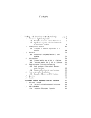

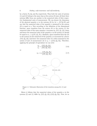
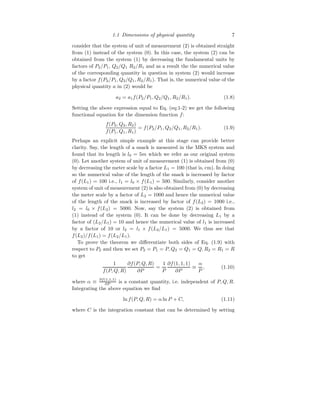
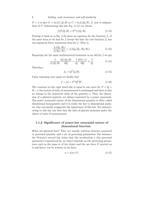
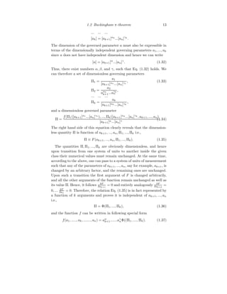
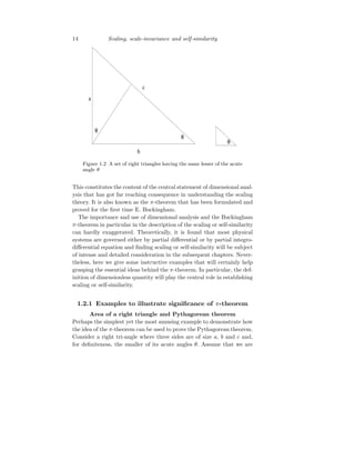
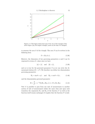
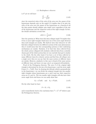
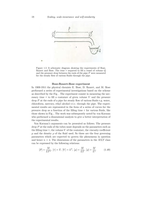
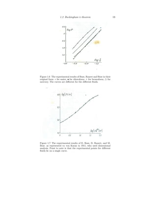
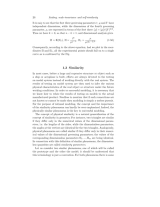
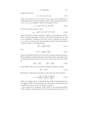
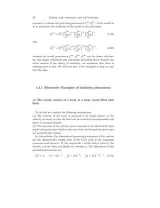
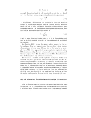
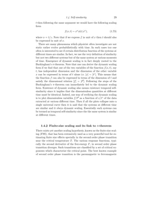
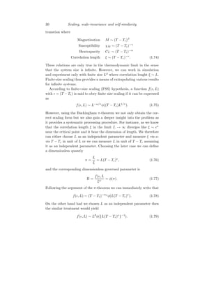
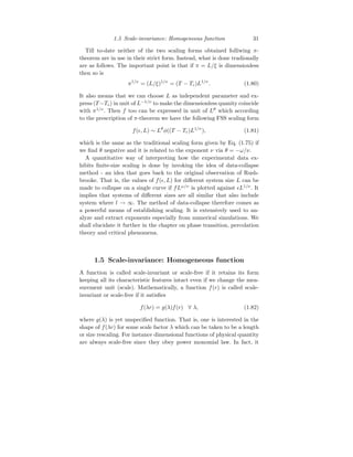
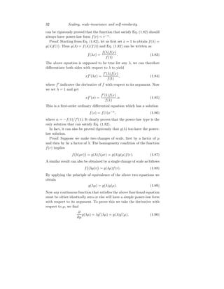
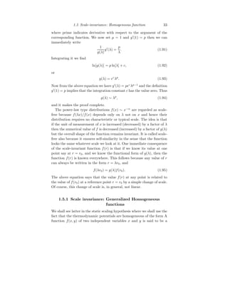
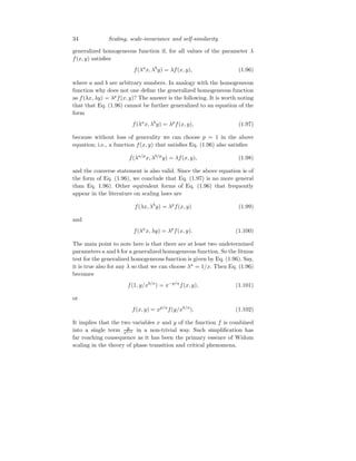
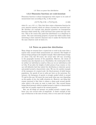
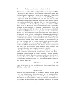
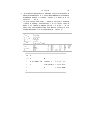
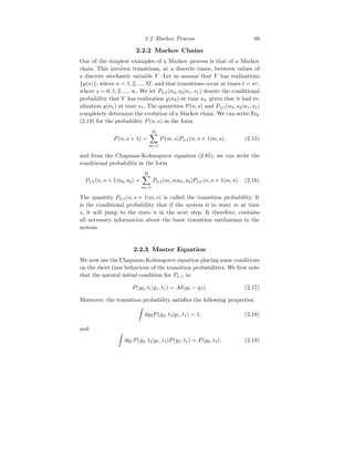
![50 Stochastic process, random walk and diffusion
We assume now that the transition probability from a state y1 to a
different state y2 in a sufficiently short time interval t2 − t1 = ∆t is
proportional to ∆t; thus
P(y2, t + ∆t|y1, t) = Aδ(y2 − y1) + ∆tω(y1 → y2; t) + O((∆t)2
), (2.20)
where ω(y1 → y2; t) is the transition probability per unit time. The
first term on the right hand side represents the probability that the
random variable remains in y1 during the interval ∆t.; the factor A
is determined by the normalization condition Eq. (2.17) in Eq. (6.19).
That is, we integrate Eq. (6.19) with respect to y2 for which the left
hand side is equal to one and the right hand side is A + ∆ta(y1) where
a(y1) =
R
dy2ω(y1 → y2; t)
A = 1 − ∆ta(y1), (2.21)
is the probability that no transition occurs during the time interval
Deltat. We now write the Chapman-Kolmogorov equation Eq. (2.85),
setting y3 = y, t3 = t + ∆t, y2 = y′
, t2 = t to obtain
P(y, t + ∆t|y1, t1) =
Z
dy′
P(y, t + ∆t|y′
, t)P(y′
, t|y1, t1). (2.22)
We then expand the right hand side to first order in ∆t using Eq. (6.19)
and find the following:
P(y, t + ∆t|y1, t1) =
Z
dy′
[Aδ(y − y′
) + ∆tω(y′
−→ y)]P(y′
, t|y1, t1)
=
Z
dy′
[1 − ∆ta(y′
)]δ(y′
− y)P(y′
, t|y1, t1) (2.23)
+ ∆t
Z
dy′
ω(y′
−→ y)]P(y′
, t|y1, t1).
Further manipulation gives:
P(y, t + ∆t|y1, t1) − P(y, t|y1, t1)
∆t
= −
Z
dy′
a(y′
)δ(y′
− y)P(y′
, t|y1, t1)
+
Z
dy′
ω(t′
−→ y)]P(y′
, t|y1, t1),
where a(y) =
R
dsω(y −→ s, t) and hence
∂P(y, t|y1, t1)
∂t
= −
Z
dsω(y → s; t)P(y, t|y1, t1)
+
Z
dsω(s → y, t)P(s, t|y1, t1). (2.24)](https://image.slidesharecdn.com/nesmbookkhm-260822092903-d508b559/85/Comprehensive-Study-of-Statistical-Mechanics-in-Non-Equilibrium-Phenomena-58-320.jpg)