Comprehensive Overview of Problem Solving, Search, and Optimization in Artificial Intelligence
Detailed exploration of AI problem formulation, state-space representation, uninformed and informed search algorithms, heuristic functions, local search methods, game playing strategies, and constraint satisfaction problems.
Comprehensive Overview of Problem Solving, Search, and Optimization in Artificial Intelligence
1.
PCIT402 : ArtificialIntelligence
Sanjivani Rural Education Society’s
Sanjivani College of Engineering, Kopargaon-423603
(An Autonomous Institute Affiliated to Savitribai Phule Pune University, Pune)
NAAC ‘A’ Grade Accredited, ISO 9001:2015 Certified
Department of Information Technology
(UG Course: NBA Accredited)
Mr. R. N. Kankrale
Assistant Professor
2.
Unit-II PROBLEM SOLVING,SEARCH, AND OPTIMIZATION
Artificial Intelligence – Overview Mr. R. N. Kankrale Department of Information Technology
State-space representation and problem formulation
Uninformed search: BFS, DFS, Uniform Cost Search, Iterative Deepening Search
Informed search: Greedy Best-First Search, A* Search, AO* Search (overview)
Heuristic functions, admissibility, and consistency
Local search: Hill Climbing, Simulated Annealing, Genetic Algorithms (overview)
Game playing: Minimax Search and Alpha-Beta Pruning
Constraint Satisfaction Problems (CSP): N-Queens, Map Coloring
Illustrative examples: Water Jug Problem,8-Puzzle, Route Finding, Vacuum Cleaner
World, Tic-Tac-Toe
3.
Unit-II PROBLEM SOLVING,SEARCH, AND OPTIMIZATION
Artificial Intelligence – Overview Mr. R. N. Kankrale Department of Information Technology
State-space representation and problem formulation
What is Problem Formulation?
Problem formulation is the process of describing a problem in a way that an AI agent can solve it
systematically.
Components of Problem Formulation
Every AI search problem is defined using five components.
Five essential components
Initial State – where the agent starts.
Actions / Operators – what the agent can do.
Transition Model – what happens after an action.
Goal Test – how we know the goal is reached.
Path Cost – how much a solution costs.
4.
Unit-II PROBLEM SOLVING,SEARCH, AND OPTIMIZATION
Artificial Intelligence – Overview Mr. R. N. Kankrale Department of Information Technology
State-space representation and problem formulation
What is State-Space Representation?
After formulating the problem, AI represents all possible situations as a state space.
Definition
State-space representation is a graph/tree containing all possible states reachable
from the initial state using allowed actions.
Think of it as:
Nodes = states
Edges = actions
5.
Unit-II PROBLEM SOLVING,SEARCH, AND OPTIMIZATION
Artificial Intelligence – Overview Mr. R. N. Kankrale Department of Information Technology
State-space representation and problem formulation
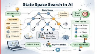
What Is State Space Search in AI?
State space search in artificial intelligence is a problem-solving technique used to find a
sequence of actions that transforms an initial state into a goal state. It represents all possible
states of a problem and explores them systematically to identify a valid solution path. State
space search is used in AI for solving puzzles, planning tasks, and decision-making
problems.
6.
Unit-II PROBLEM SOLVING,SEARCH, AND OPTIMIZATION
Artificial Intelligence – Overview Mr. R. N. Kankrale Department of Information Technology
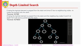
State-space representation and problem formulation
7.
Unit-II PROBLEM SOLVING,SEARCH, AND OPTIMIZATION
Artificial Intelligence – Overview Mr. R. N. Kankrale Department of Information Technology
State-space representation and problem formulation
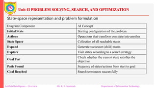
Diagram Component AI Concept
Initial State Starting configuration of the problem
Actions Operations that transform one state into another
State Space Collection of all reachable states
Expand Generate successor (child) states
Explore Visit states according to a search strategy
Goal Test
Check whether the current state satisfies the
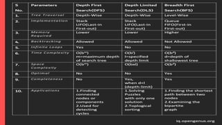
objective
Path Found Sequence of states/actions from start to goal
Goal Reached Search terminates successfully
8.
State Space Search
ArtificialIntelligence – Overview Mr. R. N. Kankrale Department of Information Technology
• “It is complete set of states including start and goal states, where the answer of the
problem is to be searched”.
• Problem:
• “It is the question which is to be solved. For solving the problem it needs to be
precisely defined. The definition means, defining the start state, goal state, other
valid states and transitions”.
• A state space representation allows for the formal definition of a problem which
makes the movement from initial state to the goal state quite easily.
• So we can say that various problems like planning, learning, theorem proving etc.
are all essentially search problems only.
• State space search is a process used in the field of computer science, including
artificial intelligence(AI), in which successive configurations or states of an instance
are considered, with the goal of finding a goal state with a desired property.
9.
Example
Artificial Intelligence –Overview Mr. R. N. Kankrale Department of Information Technology
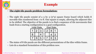
• The states of 8 tile puzzle are the different permutations of the tiles within frame.
• Lets do a standard formulation of this problem now.
• The eight tile puzzle problem formulation:
• The eight tile puzzle consist of a 3 by 3 (3*3) square frame board which holds 8
movable tiles numbered from 1 to 8. One square is empty, allowing the adjacent tiles
to be shifted. The objective of the puzzle is to find a sequence of tile movements that
leads from a starting configuration to a goal configuration.
10.
Standard Formulation
Artificial Intelligence– Overview Mr. R. N. Kankrale Department of Information Technology
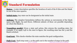
• States: A state description specifies the location of each of the 8 tiles and the blank
in one of the nine squares.
• Initial state: Any state can be designated as the initial state.
• Actions: The simplest formulation defines the actions as movements of the blank
space Left, Right, Up and Down. Different subsets of these are possible depending
on where the blank is.
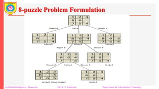
• Transition model: Given a state and action, this returns the resulting state; for
example, if we apply Left to the start in figure, the resulting state has the 5 and the
blank switched.
• Goal test: This checks whether the state matches the goal configuration.
• Path Cost: Each step costs 1, so the path cost is the number of steps in the path.
11.
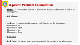
8-puzzle Problem Formulation
ArtificialIntelligence – Overview Mr. R. N. Kankrale Department of Information Technology
• States: It specifies the location of each of the 8 tiles and the blank in one of the
nine squares.
• Initial state:
• Actions: It generate legal states that result from trying the four actions;
➢Blank moves left
➢Blank moves right
➢Blank moves up
➢Blank moves down
• Goal test:
• Path Cost: Each step costs 1, so the path cost is the number of steps in the path.
Applications of StateSpace Search
Artificial Intelligence – Overview Mr. R. N. Kankrale Department of Information Technology
•State space search algorithms are used in various fields, such as robotics, game playing,
computer networks, operations research, bioinformatics, cryptography, and supply
chain management. In artificial intelligence, state space search algorithms can solve
problems like pathfinding, planning, and scheduling.
•They are also useful in planning robot motion and finding the best sequence of actions
to achieve a goal. In games, state space search algorithms can help determine the best
move for a player given a particular game state.
•State space search algorithms can optimize routing and resource allocation in computer
networks and operations research.
•In Bioinformatics, state space search algorithms can help find patterns in biological
data and predict protein structures.
•In Cryptography, state space search algorithms are used to break codes and find
cryptographic keys.
14.
Unit-II PROBLEM SOLVING,SEARCH, AND OPTIMIZATION
Artificial Intelligence – Overview Mr. R. N. Kankrale Department of Information Technology
State-space representation and problem formulation
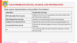
Algorithm Exploration Strategy
BFS (Breadth-First Search)
Explores level by level; guarantees the shortest path when
all actions have equal cost.
DFS (Depth-First Search) Explores one branch deeply before backtracking.
Uniform Cost Search (UCS) Expands the node with the lowest accumulated path cost.
Greedy Best-First Search
Chooses the node that appears closest to the goal based on a
heuristic.
A*
Uses both the path cost and a heuristic estimate to choose
the next node.
15.
Unit-II PROBLEM SOLVING,SEARCH, AND OPTIMIZATION
Artificial Intelligence – Overview Mr. R. N. Kankrale Department of Information Technology
State-space representation and problem formulation
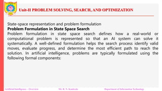
Problem Formulation in State Space Search
Problem formulation in state space search defines how a real-world or
computational problem is represented so that an AI system can solve it
systematically. A well-defined formulation helps the search process identify valid
moves, evaluate progress, and determine the most efficient path to reach the
solution. In artificial intelligence, problems are typically formulated using the
following formal components:
16.
Unit-II PROBLEM SOLVING,SEARCH, AND OPTIMIZATION
Artificial Intelligence – Overview Mr. R. N. Kankrale Department of Information Technology
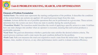
Elements of Problem Formulation
•Initial State: The initial state represents the starting configuration of the problem. It describes the condition
of the system before any actions are applied. All search processes begin from this state.
•Actions: Actions define the set of possible operations that can be performed on a given state. These actions
determine how the system can move from one state to another during the search process.
•Transition Model: The transition model describes the result of applying a specific action to a state. It defines
how one state changes into another when an operator is executed, ensuring that each action produces a
predictable outcome.
•Goal Test: The goal test determines whether a particular state satisfies the desired solution criteria. The
search process continues until a state meets the goal condition defined for the problem.
•Path Cost: Path cost measures the total cost required to reach a state from the initial state. It may represent
distance, time, number of moves, or any other performance metric used to evaluate solution efficiency.
17.
Unit-II PROBLEM SOLVING,SEARCH, AND OPTIMIZATION
Artificial Intelligence – Overview Mr. R. N. Kankrale Department of Information Technology
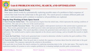
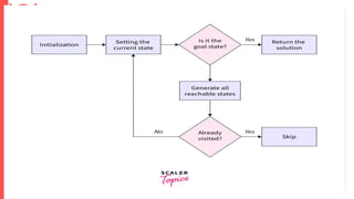
How State Space Search Works
State space search works by systematically exploring possible states of a problem to find a sequence of
actions that leads from the initial state to the goal state. The search process evaluates different paths and
selects valid transitions until a solution is reached or all possibilities are explored.
Step-by-Step Working of State Space Search
1. Start From the Initial State - The search process begins from the initial state, which represents the starting condition of
the problem. This state acts as the root of the search process.
2. Generate Possible Successor States - The system applies valid operators (actions) to the current state to generate new
states. These newly generated states are called successor states and represent possible progress toward the solution.
3. Explore the State Space - The search algorithm evaluates the generated states and selects one or more states for further
exploration. The method used to explore states depends on the chosen search strategy, such as breadth-first search or depth-
first search.
4. Check the Goal State - Each newly generated state is tested to determine whether it satisfies the goal condition. If the
goal test is successful, the search process terminates.
5. Track the Solution Path - Once the goal state is reached, the sequence of actions taken from the initial state to the goal
state is recorded. This sequence represents the solution to the problem.
If the goal state is not found, the search continues by exploring remaining states in the in the state space. This step-by-step
exploration enables AI systems to solve complex problems by evaluating multiple possible paths systematically.
18.
Unit-II PROBLEM SOLVING,SEARCH, AND OPTIMIZATION
Artificial Intelligence – Overview Mr. R. N. Kankrale Department of Information Technology
19.
Unit-II PROBLEM SOLVING,SEARCH, AND OPTIMIZATION
Artificial Intelligence – Overview Mr. R. N. Kankrale Department of Information Technology
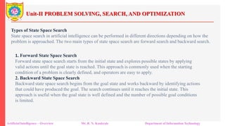
Types of State Space Search
State space search in artificial intelligence can be performed in different directions depending on how the
problem is approached. The two main types of state space search are forward search and backward search.
1. Forward State Space Search
Forward state space search starts from the initial state and explores possible states by applying
valid actions until the goal state is reached. This approach is commonly used when the starting
condition of a problem is clearly defined, and operators are easy to apply.
2. Backward State Space Search
Backward state space search begins from the goal state and works backward by identifying actions
that could have produced the goal. The search continues until it reaches the initial state. This
approach is useful when the goal state is well defined and the number of possible goal conditions
is limited.
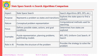
20.
State Space Searchvs Search Algorithms Comparison
Artificial Intelligence – Overview Mr. R. N. Kankrale Department of Information Technology
Aspect State Space Search Search Algorithms (BFS, DFS, etc.)
Purpose Represents a problem as states and transitions
Explores the state space to find a
solution
Nature Conceptual problem representation
Computational methods used for
searching
Focus
Defines possible states, actions, and goal
conditions
Determines how states are
explored
Examples
Puzzle representation, planning problems,
pathfinding models
BFS, DFS, Uniform Cost Search, A*
Search
Role in AI Provides the structure of the problem
Provides the strategy to solve the
problem
21.
Uninformed Search Strategies
❑Points to remember:
➢ Search without information.
➢ No prior knowledge.
➢ Time consuming.
➢ More complexity (time as well as
space)
❑ Uninformed Search Strategies:
➢ BFS (Breadth First Search)
➢ DFS (Depth First Search)
➢ UCS (Uniform Cost Search)
➢ DLS (Depth Limited Search)
➢ Iterative deepening DFS
➢ Bidirectional search
Dept of Information Technology
8/25/2026
22.
Breadth-first Search:
Artificial Intelligence– Unit-II Mr. R. N. Kankrale Department of Information Technology
Breadth first search
• Traversal means visiting all the nodes of a graph. Breadth First Traversal or
Breadth First Search is a recursive algorithm for searching all the vertices of
a graph or tree data structure.
BFS algorithm
A standard BFS implementation puts each vertex of the graph into one of two
categories:
1.Visited
2.Not Visited
The purpose of the algorithm is to mark each vertex as visited while avoiding cycles.
23.
Breadth-first Search:
Artificial Intelligence– Unit-II Mr. R. N. Kankrale Department of Information Technology
The algorithm works as follows:
1.Start by putting any one of the graph's vertices at the back of a queue.
2.Take the front item of the queue and add it to the visited list.
3.Create a list of that vertex's adjacent nodes. Add the ones which aren't in the
visited list to the back of the queue.
4.Keep repeating steps 2 and 3 until the queue is empty.
24.
Breadth-first Search:
Artificial Intelligence– Unit-II Mr. R. N. Kankrale Department of Information Technology
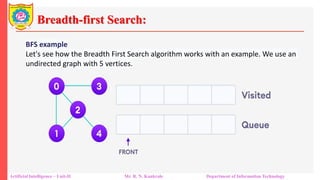
BFS example
Let's see how the Breadth First Search algorithm works with an example. We use an
undirected graph with 5 vertices.
25.
Breadth-first Search:
Artificial Intelligence– Unit-II Mr. R. N. Kankrale Department of Information Technology
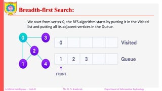
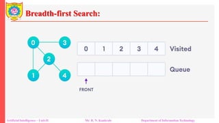
We start from vertex 0, the BFS algorithm starts by putting it in the Visited
list and putting all its adjacent vertices in the Queue.
26.
Breadth-first Search:
Artificial Intelligence– Unit-II Mr. R. N. Kankrale Department of Information Technology
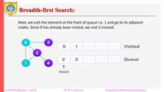
Next, we visit the element at the front of queue i.e. 1 and go to its adjacent
nodes. Since 0 has already been visited, we visit 2 instead.
27.
Breadth-first Search:
Artificial Intelligence– Unit-II Mr. R. N. Kankrale Department of Information Technology
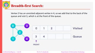
Vertex 2 has an unvisited adjacent vertex in 4, so we add that to the back of the
queue and visit 3, which is at the front of the queue.
Breadth-first Search:
Artificial Intelligence– Unit-II Mr. R. N. Kankrale Department of Information Technology
BFS Algorithm Steps:
1.Initialize:
•Create an empty list visited to track visited nodes.
•Create a queue (use list or deque) and add the starting node to both
visited and the queue.
2.Repeat while the queue is not empty:
•Dequeue (remove) the front node from the queue and process it (e.g.,
print it).
•For each neighbor of the current node:
•If the neighbor has not been visited, add it to both visited and the queue.
3.End when the queue becomes empty.
Breadth-first Search:
Artificial Intelligence– Unit-II Mr. R. N. Kankrale Department of Information Technology
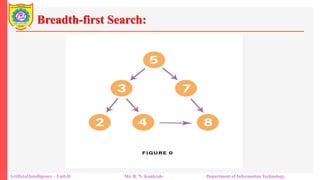
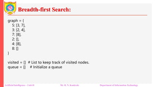
graph = {
5: [3, 7],
3: [2, 4],
7: [8],
2: [],
4: [8],
8: []
}
visited = [] # List to keep track of visited nodes.
queue = [] # Initialize a queue
33.
Breadth-first Search:
Artificial Intelligence– Unit-II Mr. R. N. Kankrale Department of Information Technology
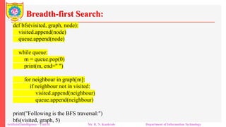
def bfs(visited, graph, node):
visited.append(node)
queue.append(node)
while queue:
m = queue.pop(0)
print(m, end=" ")
for neighbour in graph[m]:
if neighbour not in visited:
visited.append(neighbour)
queue.append(neighbour)
print("Following is the BFS traversal:")
bfs(visited, graph, 5)
34.
Breadth-first Search:
Artificial Intelligence– Unit-II Mr. R. N. Kankrale Department of Information Technology
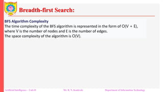
BFS Algorithm Complexity
The time complexity of the BFS algorithm is represented in the form of O(V + E),
where V is the number of nodes and E is the number of edges.
The space complexity of the algorithm is O(V).
35.
Breadth-first Search:
Artificial Intelligence– Unit-II Mr. R. N. Kankrale Department of Information Technology
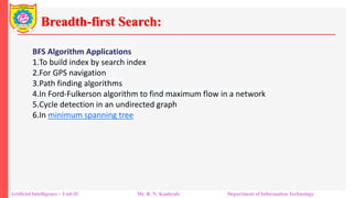
BFS Algorithm Applications
1.To build index by search index
2.For GPS navigation
3.Path finding algorithms
4.In Ford-Fulkerson algorithm to find maximum flow in a network
5.Cycle detection in an undirected graph
6.In minimum spanning tree
36.
Depth-First Search
Artificial Intelligence– Unit-II Mr. R. N. Kankrale Department of Information Technology
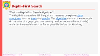
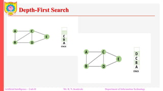
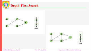
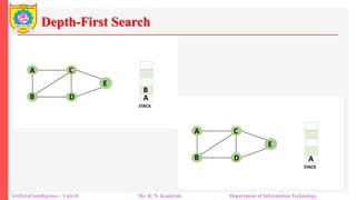
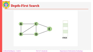
What is a Depth-First Search Algorithm?
The depth-first search or DFS algorithm traverses or explores data
structures, such as trees and graphs. The algorithm starts at the root node
(in the case of a graph, you can use any random node as the root node)
and examines each branch as far as possible before backtracking.
37.
Depth-First Search
Artificial Intelligence– Unit-II Mr. R. N. Kankrale Department of Information Technology
When a dead-end occurs in any iteration, the Depth First Search (DFS)
method traverses a network in a deathward motion and uses a stack data
structure to remember to acquire the next vertex to start a search.
38.
Depth-First Search
Artificial Intelligence– Unit-II Mr. R. N. Kankrale Department of Information Technology
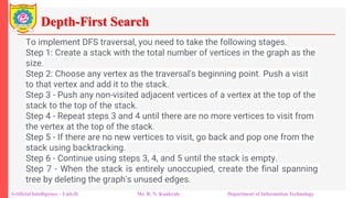
To implement DFS traversal, you need to take the following stages.
Step 1: Create a stack with the total number of vertices in the graph as the
size.
Step 2: Choose any vertex as the traversal's beginning point. Push a visit
to that vertex and add it to the stack.
Step 3 - Push any non-visited adjacent vertices of a vertex at the top of the
stack to the top of the stack.
Step 4 - Repeat steps 3 and 4 until there are no more vertices to visit from
the vertex at the top of the stack.
Step 5 - If there are no new vertices to visit, go back and pop one from the
stack using backtracking.
Step 6 - Continue using steps 3, 4, and 5 until the stack is empty.
Step 7 - When the stack is entirely unoccupied, create the final spanning
tree by deleting the graph's unused edges.
Depth-First Search
Artificial Intelligence– Unit-II Mr. R. N. Kankrale Department of Information Technology
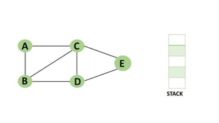
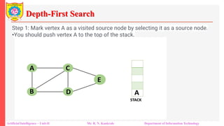
Step 1: Mark vertex A as a visited source node by selecting it as a source node.
•You should push vertex A to the top of the stack.
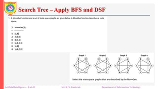
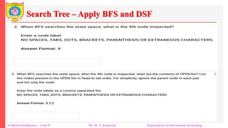
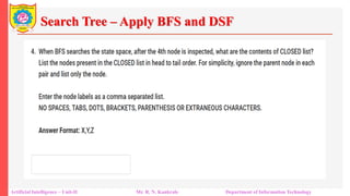
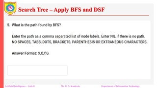
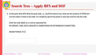
Search Tree –Apply BFS and DSF
Artificial Intelligence – Unit-II Mr. R. N. Kankrale Department of Information Technology
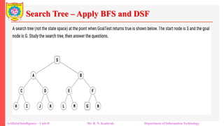
46.
Search Tree –Apply BFS and DSF
Artificial Intelligence – Unit-II Mr. R. N. Kankrale Department of Information Technology
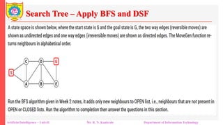
47.
Search Tree –Apply BFS and DSF
Artificial Intelligence – Unit-II Mr. R. N. Kankrale Department of Information Technology
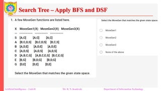
48.
Search Tree –Apply BFS and DSF
Artificial Intelligence – Unit-II Mr. R. N. Kankrale Department of Information Technology
49.
Search Tree –Apply BFS and DSF
Artificial Intelligence – Unit-II Mr. R. N. Kankrale Department of Information Technology
50.
Search Tree –Apply BFS and DSF
Artificial Intelligence – Unit-II Mr. R. N. Kankrale Department of Information Technology
51.
Search Tree –Apply BFS and DSF
Artificial Intelligence – Unit-II Mr. R. N. Kankrale Department of Information Technology
52.
Search Tree –Apply BFS and DSF
Artificial Intelligence – Unit-II Mr. R. N. Kankrale Department of Information Technology
53.
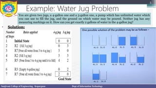
Example: Water JugProblem
5
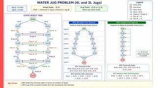
You are given two jugs, a 4-gallon one and a 3-gallon one, a pump which has unlimited water which
you can use to fill the jug, and the ground on which water may be poured. Neither jug has any
measuring markings on it. How can you get exactly 2 gallons of water in the 4-gallon jug?
• Solution:
Sanjivani College of Engineering, Kopargaon Dept of Information Technology
54.
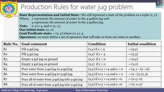
Production Rules forwater jug problem
6
Rule No. Goal comment Condition Initial condition
R1 Fill 4-gal jug (x,y) if x < 4 → (4,y)
R2 Fill 3-gal jug (x,y) if y < 3 → (x,3)
R3 Empty 4-gal jug on ground (x,y) if x > 0 → (0,y)
R4 Empty 3-gal jug on ground (x,y) if y > 0 → (x,0)
R5 Pour water from 3-gal jug to 4-gal jug (x,y) if x+y >=4 and y > 0 → (4, y - (4 - x))
R6 Pour water from 4-gal jug to 3-gal jug (x,y) if x+y >=3 and x > 0 → (x - (3-y), 3)
R7 Pour all of water from 3-gal jug into 4-gal jug (x,y) if x+y <=4 and y >0 → (x+y, 0)
R8 Pour all of water from 4-gal jug into 3-gal jug (x,y) if x+y <=3 and x >0 → (0, x+y)
Sanjivani College of Engineering, Kopargaon Dept of Information Technology
State Representation and Initial State : We will represent a state of the problem as a tuple (x, y).
Where, x represents the amount of water in the 4-gallon jug and
y represents the amount of water in the 3-gallon jug.
Note: 0 ≤x≤ 4, and 0 ≤y ≤3.
Our initial state: (0, 0)
Goal Predicate state: = (2, y) where 0≤ y≤ 3.
Operators: we must define a set of operators that will take us from one state to another;
55.
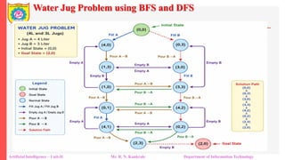
Water Jug Problemusing BFS and DFS
Artificial Intelligence – Unit-II Mr. R. N. Kankrale Department of Information Technology
56.
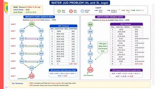
Water Jug Problemusing BFS and DFS
Artificial Intelligence – Unit-II Mr. R. N. Kankrale Department of Information Technology
57.
Water Jug Problemusing BFS and DFS
Artificial Intelligence – Unit-II Mr. R. N. Kankrale Department of Information Technology
58.
Depth Limited Search
ArtificialIntelligence – Unit-II Mr. R. N. Kankrale Department of Information Technology
Depth limited search is the new search algorithm for uninformed search. The
unbounded tree problem happens to appear in the depth-first search algorithm, and it
can be fixed by imposing a boundary or a limit to the depth of the search domain. We
will say that this limit as the depth limit, making the DFS search strategy more refined
and organized into a finite loop. We denote this limit by l, and thus this provides the
solution to the infinite path problem that originated earlier in the DFS algorithm. Thus,
Depth limited search can be called an extended and refined version of the DFS
algorithm. In a nutshell, we can say that to avoid the infinite loop status while executing
the codes, and depth limited search algorithm is being executed into a finite set of depth
called depth limit.
59.
Depth Limited Search
ArtificialIntelligence – Unit-II Mr. R. N. Kankrale Department of Information Technology
Algorithm
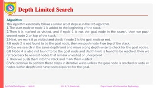
This algorithm essentially follows a similar set of steps as in the DFS algorithm.
1.The start node or node 1 is added to the beginning of the stack.
2.Then it is marked as visited, and if node 1 is not the goal node in the search, then we push
second node 2 on top of the stack.
3.Next, we mark it as visited and check if node 2 is the goal node or not.
4.If node 2 is not found to be the goal node, then we push node 4 on top of the stack.
5.Now we search in the same depth limit and move along depth-wise to check for the goal nodes.
6.If Node 4 is also not found to be the goal node and depth limit is found to be reached, then we
retrace back to nearest nodes that remain unvisited or unexplored.
7.Then we push them into the stack and mark them visited.
8.We continue to perform these steps in iterative ways unless the goal node is reached or until all
nodes within depth limit have been explored for the goal.
60.
Depth Limited Search
ArtificialIntelligence – Unit-II Mr. R. N. Kankrale Department of Information Technology
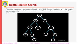
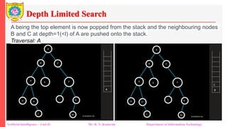
Consider the given graph with Depth Limit(l)=2, Target Node=H and the given
source node=A
61.
Depth Limited Search
ArtificialIntelligence – Unit-II Mr. R. N. Kankrale Department of Information Technology
A being the top element is now popped from the stack and the neighbouring nodes
B and C at depth=1(<l) of A are pushed onto the stack.
Traversal: A
62.
Depth Limited Search
ArtificialIntelligence – Unit-II Mr. R. N. Kankrale Department of Information Technology
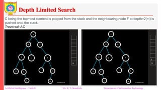
C being the topmost element is popped from the stack and the neighbouring node F at depth=2(=l) is
pushed onto the stack.
Traversal: AC
63.
Depth Limited Search
ArtificialIntelligence – Unit-II Mr. R. N. Kankrale Department of Information Technology
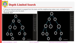
F being the topmost element is popped from the stack and the neighbouring nodes I and J at depth=3(>l)
will not be pushed onto the stack.
Traversal: ACF
64.
Depth Limited Search
ArtificialIntelligence – Unit-II Mr. R. N. Kankrale Department of Information Technology
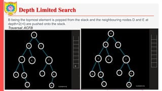
B being the topmost element is popped from the stack and the neighbouring nodes D and E at
depth=2(=l) are pushed onto the stack.
Traversal: ACFB
65.
Depth Limited Search
ArtificialIntelligence – Unit-II Mr. R. N. Kankrale Department of Information Technology
E being the topmost element is popped from the stack and since E has no neighbouring nodes, no
nodes are pushed onto the stack.
Traversal: ACFBE
D being the topmost element is popped from the stack and the neighbouring nodes G and H at
depth=3(>l) will not be pushed onto the stack.
Traversal: ACFBED
66.
Depth Limited Search
ArtificialIntelligence – Unit-II Mr. R. N. Kankrale Department of Information Technology
Measures of Performance
Completeness: DLS search algorithm is complete if the solution is above the
depth-limit.
Time Complexity: Time complexity of DLS algorithm is O(b^l) where b is known
as the branching factor (number of children at each node) and l is the given
depth limit.
Space Complexity: Space complexity of DLS algorithm is O(bxl) where b is
known as the branching factor (number of children at each node) and l is the
given depth limit.
Optimal: Even if l>d, depth-limited search is not ideal.
67.
Depth Limited Search
ArtificialIntelligence – Unit-II Mr. R. N. Kankrale Department of Information Technology
Advantages of Depth Limited Search
1.Depth limited search is more efficient than DFS, using less time and memory.
2.If a solution exists, DFS guarantees that it will be found in a finite amount of time.
3.To address the drawbacks of DFS, we set a depth limit and run our search
technique repeatedly through the search tree.
4.DLS has applications in graph theory that are highly comparable to DFS.
Disadvantages of Depth Limited Search
1.For this method to work, it must have a depth limit.
2.If the target node does not exist inside the chosen depth limit, the user will be
forced to iterate again, increasing execution time.
3.If the goal node does not exist within the specified limit, it will not be discovered.
Iterative Deepening DepthFirst Search
Artificial Intelligence – Unit-II Mr. R. N. Kankrale Department of Information Technology
70.
Iterative Deepening DepthFirst Search
Artificial Intelligence – Unit-II Mr. R. N. Kankrale Department of Information Technology
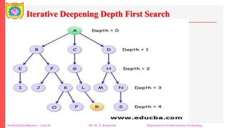
Here in the given tree, the starting node is A and the depth initialized to 0.
The goal node is R where we have to find the depth and the path to reach it.
In this example, we consider the tree as a finite tree, while we can consider
the same procedure for the infinite tree as well. We knew that in the
algorithm of IDDFS we first do DFS till a specified depth and then increase the
depth at each loop. This special step forms the part of DLS or Depth Limited
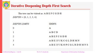
Search. Thus the following traversal shows the IDDFS search.
71.
Iterative Deepening DepthFirst Search
Artificial Intelligence – Unit-II Mr. R. N. Kankrale Department of Information Technology
72.
Iterative Deepening DepthFirst Search
Artificial Intelligence – Unit-II Mr. R. N. Kankrale Department of Information Technology
Advantages
•IDDFS gives us the hope to find the solution if it exists in the tree.
•When the solutions are found at the lower depths say n, then the algorithm proves to be efficient
and in time.
•The great advantage of IDDFS is found in-game tree searching where the IDDFS search operation
tries to improve the depth definition, heuristics, and scores of searching nodes so as to enable
efficiency in the search algorithm.
•Another major advantage of the IDDFS algorithm is its quick responsiveness. The early results
indications are a plus point in this algorithm. This followed up with multiple refinements after the
individual iteration is completed.
•Though the work is done here is more yet the performance of IDDFS is better than single BFS and
DFS operating exclusively.
•Space and time complexities are expressed as: O(d) and here d is defined as goal depth.
•Let us consider the run time of IDDFS. Let say b>l where b is branching factor and l is the depth
limit. Then next we search the goal node under the bound k. On the depth k, we say there may
be bknodes that are only generated once. Similarly, the nodes at the depth limit k-1 is twice and
thrice for k-2 depth. Thus the node generated at depth l is k times.
73.
Iterative Deepening DepthFirst Search
Artificial Intelligence – Unit-II Mr. R. N. Kankrale Department of Information Technology
Disadvantages
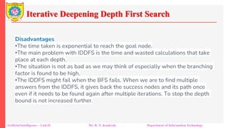
•The time taken is exponential to reach the goal node.
•The main problem with IDDFS is the time and wasted calculations that take
place at each depth.
•The situation is not as bad as we may think of especially when the branching
factor is found to be high.
•The IDDFS might fail when the BFS fails. When we are to find multiple
answers from the IDDFS, it gives back the success nodes and its path once
even if it needs to be found again after multiple iterations. To stop the depth
bound is not increased further.
74.
Bidirectional Search
Artificial Intelligence– Unit-II Mr. R. N. Kankrale Department of Information Technology
Bidirectional search is a graph search where unlike Breadth First
search and Depth First Search, the search begins simultaneously
from Source vertex and Goal vertex and ends when the two
searches meet somewhere in between in the graph. This is thus
especially used for getting results in a fraction of the time taken
by both DFS and FS searches. The search from the initial node is
forward search while that from the goal node is backwards. It is
also based on heuristic search meaning finding the shortest
path to goal optimally.
75.
Bidirectional Search
Artificial Intelligence– Unit-II Mr. R. N. Kankrale Department of Information Technology
Heuristic refers to the concept of finding the shortest path from the current node in
the graph to the goal node. The search always takes the shortest path to the goal
node. This principle is used in a bidirectional heuristic search. The only difference
being the two simultaneous searches from the initial point and from goal vertex. The
main idea behind bidirectional searches is to reduce the time taken for search
drastically.
This happens when both searches happen simultaneously from the initial node depth
or breadth-first and backwards from goal nodes intersecting somewhere in between
of the graph. Now the path traverses through the initial node through the intersecting
point to goal vertex is the shortest path found because of this search. This is the
shortest path and found in a fraction of time taken by other search algorithms.
76.
Bidirectional Search
Artificial Intelligence– Unit-II Mr. R. N. Kankrale Department of Information Technology
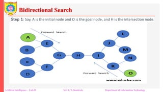
Step 1: Say, A is the initial node and O is the goal node, and H is the intersection node.
77.
Bidirectional Search
Artificial Intelligence– Unit-II Mr. R. N. Kankrale Department of Information Technology
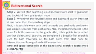
Step 2: We will start searching simultaneously from start to goal node
and backward from goal to start node.
Step 3: Whenever the forward search and backward search intersect
at one node, then the searching stops.
Thus, it is possible when both the Start node and goal node are known
and unique, separate from each other. Also, the branching factor is the
same for both traversals in the graph. Also, other points to be noted
are that bidirectional searches are complete if a breadth-first search is
used for both traversals, i.e. for both paths from start node till
intersection and from goal node till intersection.
Time and Space complexity of the bidirectional search is represented
by O(b^{d/2})
78.
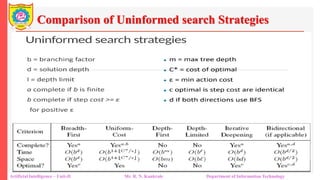
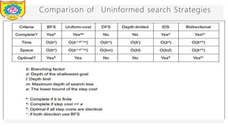
Comparison of Uninformedsearch Strategies
Artificial Intelligence – Unit-II Mr. R. N. Kankrale Department of Information Technology
79.
Searching with partialinformation Sensor-less problems, Contingency
problems.
Artificial Intelligence – Unit-II Mr. R. N. Kankrale Department of Information Technology
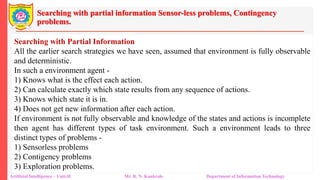
Searching with Partial Information
All the earlier search strategies we have seen, assumed that environment is fully observable
and deterministic.
In such a environment agent -
1) Knows what is the effect each action.
2) Can calculate exactly which state results from any sequence of actions.
3) Knows which state it is in.
4) Does not get new information after each action.
If environment is not fully observable and knowledge of the states and actions is incomplete
then agent has different types of task environment. Such a environment leads to three
distinct types of problems -
1) Sensorless problems
2) Contigency problems
3) Exploration problems.
80.
Searching with partialinformation
Artificial Intelligence – Unit-II Mr. R. N. Kankrale Department of Information Technology
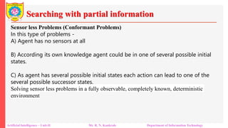
Sensor less Problems (Conformant Problems)
In this type of problems -
A) Agent has no sensors at all
B) According its own knowledge agent could be in one of several possible initial
states.
C) As agent has several possible initial states each action can lead to one of the
several possible successor states.
Solving sensor less problems in a fully observable, completely known, deterministic
environment
81.
Searching with partialinformation
Artificial Intelligence – Unit-II Mr. R. N. Kankrale Department of Information Technology
In sensor less problem agent already have predefined knowledge about its various states.
Out of these state set only one of the state is going to be initial state. Though agent has no
sensor, hence no percepts, still from its own state and action it can reach to certain
conclusion states, through which it can further reach to goal state. It means that we can
say agent can coerce (force to reach) the world to reach at a particular expected state on
his own.
Steps taken to solve the problem are as follows -
1) First agent searches for belief state instead of physical state.
[The belief state - it is a set of states representing agent's current belief about the
possible physical states it might be in. For finding such belief state agent should
have reasoning for each state it can be in, based on its original knowledge].
82.
Searching with partialinformation
Artificial Intelligence – Unit-II Mr. R. N. Kankrale Department of Information Technology
2) Initial state is belief state which can further mapped to another belief state.
3) Action is applied to belief state by taking union of the results obtained from
applying the action to each physical state in the belief state.
4) We now get a path which connects several belief states.
5) Solution is a path that leads to a belief state, all of whose members are goal
states.
Note If the physical state space has 's' states, the belief state space will have 25
belief states.
For Example
• Black ball picker robot
83.
Searching with partialinformation
Artificial Intelligence – Unit-II Mr. R. N. Kankrale Department of Information Technology
Contingency Problem
If environment is partially observable or if actions are uncertain, then agent can sense and
perceive new information after each action. This new information can lead to new problem
(or critical situation) which is called as contingency. If this situation occurs then agent needs
to plan next action to handle this contingency.
• Solving contingency problem -
1) For contingency problem one needs to form a tree, here each branch of a tree may be
selected depending upon the percepts received up to that point in the tree.
2) Then by searching and expanding previous level agent can reach to a goal.
In some situations for contingency problems we get purely sequential solutions.
Note Searching algorithm for contingency problems are more complex than algorithms we
have studied so far.
84.
Searching with partialinformation
Artificial Intelligence – Unit-II Mr. R. N. Kankrale Department of Information Technology
The agent design is also different for these problems, because agent can act before it has
found a guaranteed plan.
Agent continue to solve problem, considering new information and minimizing he
contingency by checking the output of its action. This is termed as interleaving of searching
and execution. [That is alternately search and execution is done].
For example:
Trading agent
• Special case of contingency problem: A contingency problem is called as adversarial
problem if the uncertainty is caused by the actions of another agent. (More adverse
situation).
For example -
Agent in game of chess.
85.
Searching with partialinformation
Artificial Intelligence – Unit-II Mr. R. N. Kankrale Department of Information Technology
Extreme Case of Contingency Problem
Exploration problem: When state as well as the actions of the environment are unknown
the agent must act to discover them. The interleaving of searching and execution would
be useful to solve exploration problem.
For example -
The boat driving robotic agent.
86.
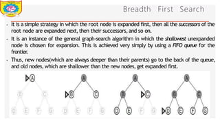
Breadth First Search
⦁It is a simple strategy in which the root node is expanded first, then all the successors of the
root node are expanded next,then their successors,and so on.
⦁ It is an instance of the general graph-search algorithm in which the shallowest unexpanded
node is chosen for expansion. This is achieved very simply by using a FIFO queue for the
frontier
.
⦁ Thus, new nodes(which are always deeper than their parents) go to the back of the queue,
and old nodes,which are shallower than the new nodes,get expanded first.
Dept of Information Technology 8/25/2026
87.
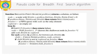
Pseudo code forBreadth First Search algorithm
Dept of Information Technology 8/25/2026
88.
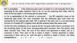
Let us checkif the BFS algorithm satisfies the 4 properties :
⦁ BFS is complete — if the shallowest goal node is at depth d,it will eventually find it after
expanding all the nodes shallower than d. (ie. As we are exploring each node, level by
level,till the last depth,it will always give the goal node)
⦁ As far as optimality of the solution is concerned — the BFS algorithm stops at the
shallowest goal found. We must remember that the shallowest goal node need not
necessarily be the optimal goal node. BFS is optimal if the path cost is a non-decreasing
function of d.Usually,BFS is applied when all the actions have the same cost.
⦁ To find the time complexity, let us assume all the non-goal nodes have b successors (b is
the branching factor of the tree), and generating each successor from the parent node
takes constant time. Then, the root of the search tree generates b nodes, and so it
consumes b time. Then each of the b nodes in depth 1 further generates b nodes,
consuming b² time, and so on, until the goal is reached in depth d. Hence, the time
complexity is;
Dept of Information Technology 8/25/2026
89.
Let us checkif the BFS algorithm satisfies the 4 properties :
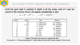
⦁ Until the goal node is reached in depth d, all the nodes until d-1 must be
stored in the memory.Hence,the space complexity is also:
Figure :The time and memory required for BFS.
We assume b = 10,the processing speed is 1 million nodes per second,and the space required is 1kB per node
Dept of Information Technology 8/25/2026
90.
Depth First Search
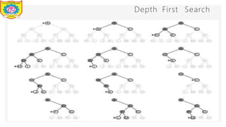
⦁It always expands the deepest node in the current frontier of the search tree.
⦁ The search proceeds immediately to the deepest level of the search tree, where
the nodes have no successors.
⦁ As those nodes are expanded, they are dropped from the frontier
, so then the
search“backs up” to the next deepest node that still has unexplored successors.
⦁ DFS uses a LIFO queue, means that, the most recently generated node is chosen
for expansion. This must be the deepest unexpanded node because it is one
deeper than its parent which, in turn, was the deepest unexpanded node when it
was selected.
Dept of Information Technology 8/25/2026
Let us checkif the DFS algorithm satisfies the 4 properties :
⦁ DFS is not complete. In the problem of traveling from Arad to Bucharest, the search agent might get
stuck in Arad — Sibiu — Arad loop forever
. The only way to avoid loopy path in DFS is to remember all
the nodes present in the path from the root to the current node. This could solve the problem of
loopy paths,but still cannot avoid redundant paths.
⦁ DFS is non-optimal in nature. DFS will explore all the left nodes first, even if node C is the optimal
solution. Suppose node K is also a solution (but a non-optimal one), DFS returns K as the optimal
solution.
⦁ Time taken by DFS depends on the depth of the entire search tree (which could be infinite, if loopy paths
are not eliminated). Even in the case of a search tree with finite depth, the time complexity will be
O(b^m), where m is the maximum depth of the search tree, which could be much larger than d (the
depth of the shallowest goal).
⦁ The main reason for the use of DFS over BFS in many areas of AI is because of its very less space
consumption. In DFS, we need to store only the nodes which are present in the path from the root to the
current node and their unexplored successors. For state space with branching factor b and maximum
depth m,DFS has space complexity of O(bm), a much better improvement over that of BFS.
Dept of Information Technology 8/25/2026
93.
Depth Limited Search
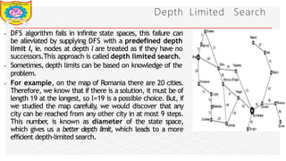
⦁DFS algorithm fails in infinite state spaces, this failure can
be alleviated by supplying DFS with a predefined depth
limit l, ie. nodes at depth l are treated as if they have no
successors.This approach is called depth limited search.
⦁ Sometimes, depth limits can be based on knowledge of the
problem.
⦁ For example, on the map of Romania there are 20 cities.
Therefore, we know that if there is a solution, it must be of
length 19 at the longest, so l=19 is a possible choice. But, if
we studied the map carefully
, we would discover that any
city can be reached from any other city in at most 9 steps.
This number
, is known as diameter of the state space,
which gives us a better depth limit, which leads to a more
efficient depth-limited search.
Dept of Information Technology 8/25/2026
94.
Let us checkif the DLS algorithm satisfies the 4 properties :
⦁ Depth-limited search solves the infinite-path problem.But the search is not complete
ifl< d.
⦁ Even if l
> d
,optimal solution is not guaranteed,as we could be eliminating some ofthesolutions atdepths> l
.
⦁ TimecomplexityisO (b^l).
⦁ SpacecomplexityisO(bl) (ItissameasDFS,onlywithrestricteddepthto l
)
.
⦁ Inf
ac
t,DFS canbeviewedasaspecial-caseofdepth-limitedsearchwithl→infinity
.
⦁ The problem with depth-limited search is to set the value of loptimally
,so as to not leaveout anysolution,aswellaskeepthetimeandspacecomplexityto aminimum.
Dept of Information Technology 8/25/2026
95.
Iterative Deepening DepthFirst Search
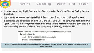
⦁ Iterative-deepening depth-first search offers a solution for the problem of finding the best
depth limit.
⦁ It gradually increases the depth first 0,then 1,then 2,and so on until a goal is found.
⦁ It combines the advantages of both BFS and DFS. Like DFS, it consumes less memory:
O(bd). Like BFS, it is complete when b is finite, and is optimal when the path cost is a
non-decreasing function of depth.Time complexity is O(b^d), similar to BFS.
Iterative-deepening search,repeatedly calling the depth-limited search while varying the depth limit in
every iteration.
Dept of Information Technology 8/25/2026
96.
Iterative Deepening DepthFirst Search
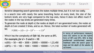
⦁ Iterative deepening search generates the states multiple times,but it is not too costly.
⦁ In a search tree with nearly the same branching factor at every level, the size of the
bottom levels are very huge compared to the top ones, hence it does not affect much if
the nodes in the top levels are generated many times.
⦁ To generate the node at depth d, the nodes at depth d-1 are generated twice, the nodes at
depth d-2 are created 3 times, and so on. Hence, the total number of nodes generated will
be;
⦁ Which has the complexity of O(b^d), the same as BFS.
For example,for d = 5 and b = 10:
⦁ n(IDS) = 50 + 400 + 3000 + 20000 + 100000 = 1,23,450
⦁ n(BFS) = 10 + 100 + 1000 + 10000 + 100000 = 1,11,110
In terms of performance measure,
since IDS seems to be the hybrid
form of BFS and DFS, IDS is the
preferred uninformed search
method when the search space is
large and the depth of the solution is
not known.
Dept of Information Technology 8/25/2026
97.
Bidirectional Search
⦁ Theidea behind the bidirectional search is to run two searches simultaneously — one
forward from the start state, and the other from the goal — hoping that the two will meet
somewhere in the middle.
⦁ It is implemented by replacing the goal test with a check to see whether the frontiers of
the two search intersect (the solution is found if they do). The check can be performed
when the node is generated,and can be done in constant time using hash tables.
⦁ The main aim of bidirectional search is to reduce the total search time. If we use BFS at
both the ends as the search algorithm, the time and space complexity will be
O(b^(d/2))(In the worst case,the two frontiers meet in the middle).
⦁ The space can be reduced if one of them is IDS, but one of the frontiers must be in the
memory to perform the check for the intersection.
Dept of Information Technology 8/25/2026
98.
Bidirectional Search
2
2
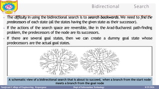
⦁ Thedifficulty in using the bidirectional search is to search backwards.We need to find the
predecessors of each state (all the states having the given state as their successor).
⦁ If the actions of the search space are reversible, like in the Arad-Bucharest path-finding
problem,the predecessors of the node are its successors.
⦁ If there are several goal states, then we can create a dummy goal state whose
predecessors are the actual goal states.
A schematic view of a bidirectional search that is about to succeed, when a branch from the start node
meets a branch from the goal node
Sanjivani College of Engineering, Kopargaon Dept of Information Technology 8/25/2026
Searching with partialinformation
⦁ What if the knowledge of the states or actions is incomplete?
⦁ That means,if the environment is not fully observable or deterministic.
⦁ Different types of incompleteness lead to three distinct problem types;
1.Sensorless problems,
2.Contingency problems,
3.Exploration problems
Dept of Information Technology 8/25/2026


 Most read