Comprehensive Introduction to Engineering Metrology: Standards and Measurement Techniques

Comprehensive Introduction to Engineering Metrology: Standards and Measurement Techniques

• 1.
  Engineering Metrology —Unit 1a Page 1 Introduction to Metrology Definition & Objectives of Metrology · Standards of Measurement · Material, Line, End and Wavelength Standards 1. Definition of Metrology DEFINITION Metrology is the science of measurement. It deals with the establishment, reproduction, conservation and transfer of units of measurement and their standards. In an engineering context, it covers the measurement of dimensions, form, surface finish, and other physical quantities of a manufactured component, ensuring interchangeability and quality of parts. The word “metrology” is derived from the Greek words metron (measure) and logos (study/science). Engineering metrology, in particular, is concerned with the application of measurement science to manufacturing and related industrial problems. 2. Objectives of Metrology The primary objectives of metrology in an industrial/production environment are: 1. To provide accuracy at minimum cost — selecting the measuring instrument and method that gives the required accuracy at the lowest possible cost. 2. To determine the process capability and ensure that it is consistent with the tolerance requirement specified on the component drawing. 3. To determine the measuring instrument capability and ensure it is adequate for its intended use (instrument error should be small compared with the tolerance to be measured, generally 1/10th rule). 4. To minimize the cost of inspection by effective and efficient utilization of available facilities and resources. 5. To reduce the cost of rejects and rework through timely detection of faulty components and processes (quality control). 6. To standardize measuring methods, i.e., to establish uniform testing procedures. 7. To maintain interchangeability of components in mass production by ensuring dimensional consistency. 8. To provide a means for evaluation of the quality of the manufactured product and to help in maintaining specified quality standards. 9. To assess the measuring instruments’ accuracy and precision so that suitable correction factors can be introduced. NOTE In short: metrology aims to achieve uniformity, accuracy, and reliability of measurements at the lowest possible
• 2.
  Engineering Metrology —Unit 1a Page 2 cost, which in turn ensures interchangeable manufacture and quality control. 3. Standards of Measurement A standard is a physical embodiment of a unit of measurement — a reference used to check or calibrate other measuring instruments. For a standard to be useful it must be permanent, easily reproducible, and stable (not affected by environmental changes such as temperature, humidity, etc.). 3.1 Material Standards DEFINITION A material standard is a physical object (a bar, block, or scale) whose length between two marked points, or between two flat end faces, represents a known, standardized unit of length. 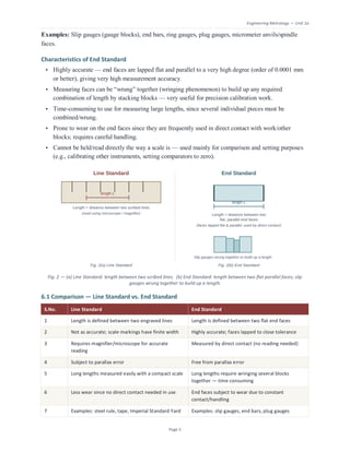Material standards are broadly divided into two types based on how the length is defined on the object: • Line Standards — length is defined as the distance between two engraved/scribed lines. • End Standards — length is defined as the distance between two flat, parallel end faces. Historically, material standards such as the Imperial Standard Yard (UK) and the International Prototype Metre (kept at the International Bureau of Weights and Measures, BIPM, Sèvres, France) were used to define the fundamental unit of length. These were bronze/platinum-iridium bars maintained under controlled conditions (0°C or 20°C, atmospheric pressure, supported at specific points called Airy points to minimize sag). 3.2 Wavelength Standards DEFINITION A wavelength standard defines the unit of length in terms of the wavelength of a specified monochromatic light source, rather than a physical artifact. Material standards, however carefully preserved, suffer from limitations: they can be damaged, they change dimensions slightly with time (due to internal stresses) and temperature, and there is only one master original, making it inconvenient for widespread comparison. To overcome this, the unit of length was redefined using light wavelength — which is a natural, indestructible, and universally reproducible standard. • 1960: The metre was redefined as 1,650,763.73 wavelengths of the orange-red radiation of Krypton- 86 in vacuum. • 1983: The metre was further redefined in terms of the speed of light — as the length of the path travelled by light in vacuum during a time interval of 1/299,792,458 of a second. • In practice, laboratories now commonly use stabilized Helium-Neon (He-Ne) laser light sources for high-precision length interferometry, since lasers give a highly monochromatic, coherent, and intense light source.
• 3.
  Engineering Metrology —Unit 1a Page 3 Advantages of Wavelength Standard over Material Standard Wavelength Standard Material Standard Not subject to damage or destruction Can be lost, damaged, or destroyed Does not change with time (perfectly reproducible) Changes dimension slightly over long periods (aging) Can be reproduced in any properly equipped laboratory — no need to refer to a single master Only one original master exists; comparison copies may introduce error Very high accuracy of length measurement (order of 0.01 micron) Comparatively less accurate; affected by temperature, support conditions Not affected by temperature/humidity variations of environment Requires strict environmental control (fixed temperature, support points) 4. 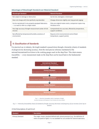Classification of Standards For practical use in industry, the length standard is passed down through a hierarchy (chain) of standards of progressively decreasing accuracy, from the most precise reference maintained at the national/international level down to the working gauges used on the shop floor. This chain ensures traceability — every measurement made on the shop floor can be traced back to the fundamental standard. Fig. 1 — Hierarchy (traceability chain) of standards of length. Accuracy decreases and frequency of use increases from top to bottom. A brief description of each level: Standard Description Primary Standard The single, master standard defined with utmost precision (e.g., the definition of metre via speed of light). It is not available for use outside the national laboratory
• 4.
  Engineering Metrology —Unit 1a Page 4 Standard Description and is used only for comparison purposes, at rare intervals. Secondary Standard An exact copy of the primary standard, kept at national/regional standards organizations (e.g. National Physical Laboratory - NPL, Bureau of Indian Standards - BIS). Used to calibrate tertiary/reference standards and for legal reference in case of dispute. Tertiary Standard Derived from secondary standards; used by instrument manufacturing companies and metrology labs as the reference for calibrating their working/inspection standards. Working Standard Used in everyday inspection and workshop practice — e.g., slip gauge sets, master scales, gauge blocks. These are checked periodically against tertiary standards. ALTERNATE CLASSIFICATION (BY DEGREE OF ACCURACY / TYPE) Standards are also classified by their physical form as: (i) Line Standard, (ii) End Standard, and (iii) Wavelength Standard — discussed in detail below. 5. Line Standard DEFINITION A Line Standard is one in which the length being measured or defined is the distance between the centres of two engraved lines on a scale, bar, or plate. Examples: Imperial Standard Yard, International Prototype Metre, engineer’s steel rule/scale, measuring tapes. Characteristics of Line Standard • Scale can be accommodated in a small space; long lengths can be measured using a relatively short, compact scale/bar with graduations. • Measurement involves the use of a microscope or magnifying lens to align with the graduation lines, hence subject to reading/parallax error. • Graduation lines have a finite thickness (~0.05 to 0.15 mm), so they themselves introduce some uncertainty; scale markings wear out with use. • Not as accurate as end standards — typical accuracy attainable is about ±0.2 mm for a metre length. • Thermal expansion effects are relatively less critical since the whole length is not always in contact/loaded. 6. End Standard DEFINITION An End Standard is one in which the length being measured or defined is the distance between two flat, parallel end faces of a bar, block, rod, or plug — measurement is taken end-to-end, not line-to-line.
• 5.
  Engineering Metrology —Unit 1a Page 5 Examples: Slip gauges (gauge blocks), end bars, ring gauges, plug gauges, micrometer anvils/spindle faces. Characteristics of End Standard • Highly accurate — end faces are lapped flat and parallel to a very high degree (order of 0.0001 mm or better), giving very high measurement accuracy. • Measuring faces can be “wrung” together (wringing phenomenon) to build up any required combination of length by stacking blocks — very useful for precision calibration work. • Time-consuming to use for measuring large lengths, since several individual pieces must be combined/wrung. • Prone to wear on the end faces since they are frequently used in direct contact with work/other blocks; requires careful handling. • Cannot be held/read directly the way a scale is — used mainly for comparison and setting purposes (e.g., calibrating other instruments, setting comparators to zero). Fig. 2 — (a) Line Standard: length between two scribed lines. (b) End Standard: length between two flat parallel faces; slip gauges wrung together to build up a length. 6.1 Comparison — Line Standard vs. End Standard S.No. Line Standard End Standard 1 Length is defined between two engraved lines Length is defined between two flat end faces 2 Not as accurate; scale markings have finite width Highly accurate; faces lapped to close tolerance 3 Requires magnifier/microscope for accurate reading Measured by direct contact (no reading needed) 4 Subject to parallax error Free from parallax error 5 Long lengths measured easily with a compact scale Long lengths require wringing several blocks together — time consuming 6 Less wear since no direct contact needed in use End faces subject to wear due to constant contact/handling 7 Examples: steel rule, tape, Imperial Standard Yard Examples: slip gauges, end bars, plug gauges
• 6.
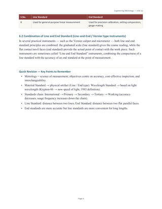
  Engineering Metrology —Unit 1a Page 6 S.No. Line Standard End Standard 8 Used for general-purpose linear measurement Used for precision calibration, setting comparators, gauge-making 6.2 Combination of Line and End Standard (Line-and-End / Vernier type instruments) In several practical instruments — such as the Vernier caliper and micrometer — both line and end standard principles are combined: the graduated scale (line standard) gives the coarse reading, while the flat contact/anvil faces (end standard) provide the actual point of contact with the work piece. Such instruments are sometimes called “Line and End Standard” instruments, combining the compactness of a line standard with the accuracy of an end standard at the point of measurement. Quick Revision — Key Points to Remember • Metrology = science of measurement; objectives centre on accuracy, cost-effective inspection, and interchangeability. • Material Standard → physical artifact (Line / End type). Wavelength Standard → based on light wavelength (Krypton-86 → now speed of light, 1983 definition). • Standards chain: International → Primary → Secondary → Tertiary → Working (accuracy decreases, usage frequency increases down the chain). • Line Standard: distance between two lines; End Standard: distance between two flat parallel faces. • End standards are more accurate but line standards are more convenient for long lengths.
• 7.
  Engineering Metrology —Unit 1b: Linear & Angular Measurement Page 1 Linear and Angular Measurements Micrometers · Height Gauges · Slip Gauges & Indian Standards · Wringing of Slip Gauges · Sine Bar · Autocollimator 1. Linear and Angular Measurement — Introduction Linear measurement deals with the measurement of length, diameter, height, or depth of a component by direct comparison with a known standard of length. It may be carried out by direct methods (steel rule, vernier caliper, micrometers, slip gauges, height gauge) or by indirect/comparative methods (dial indicators, comparators). Angular measurement deals with the determination of the angle between two lines, faces, or axes of a component, or the setting/checking of a given angle. Common methods/instruments include the bevel protractor, sine bar, sine centre, angle gauges, spirit level/clinometer, and the autocollimator. 2. Micrometers DEFINITION A micrometer is a precision linear-measuring instrument that works on the principle of a screw thread: rotation of a very accurately made screw (the spindle) inside a fixed nut converts a small linear displacement into a larger, easily readable rotary movement on a graduated thimble. 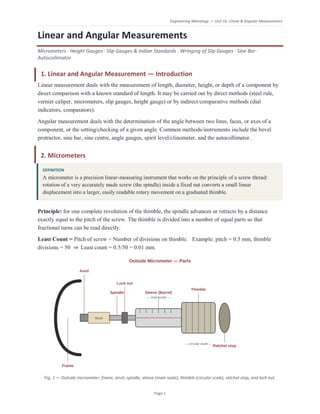Principle: for one complete revolution of the thimble, the spindle advances or retracts by a distance exactly equal to the pitch of the screw. The thimble is divided into a number of equal parts so that fractional turns can be read directly. Least Count = Pitch of screw ÷ Number of divisions on thimble. Example: pitch = 0.5 mm, thimble divisions = 50 ⇒ Least count = 0.5/50 = 0.01 mm. Fig. 1 — Outside micrometer: frame, anvil, spindle, sleeve (main scale), thimble (circular scale), ratchet stop, and lock nut.
• 8.
  Engineering Metrology —Unit 1b: Linear & Angular Measurement Page 2 2.1 Types of Micrometers • Outside Micrometer (Micrometer Caliper) — the most common type; used to measure external dimensions such as diameter or thickness of a work piece. Available in standard ranges of 25 mm (0– 25, 25–50, 50–75 mm, etc.). • Inside Micrometer — used to measure internal dimensions such as bore or hole diameters and groove widths; fitted with extension rods to cover a range of sizes. • Depth Micrometer — used to measure the depth of holes, slots, steps, and recesses; has a flat base plate instead of a frame, with the spindle extending through it. • Screw Thread Micrometer — has a V-shaped anvil and a cone-shaped spindle tip specially shaped to seat on the flanks of a screw thread, used to measure the effective (pitch) diameter of threads. • Digital / Vernier Micrometer — modern variants fitted with a digital electronic readout, or an additional vernier scale on the sleeve for finer reading down to 0.001 mm. 2.2 Parts of an Outside Micrometer Part Function Frame U/C-shaped rigid body that holds the anvil and barrel in correct alignment; often insulated with plastic grips to avoid thermal expansion from hand heat. Anvil Fixed measuring face against which the work piece rests. Spindle Moving measuring face; advances/retracts as the thimble is rotated, driven by the internal precision screw. Sleeve (Barrel) Fixed sleeve carrying the main (longitudinal) scale, graduated in mm and half-mm. Thimble Rotating sleeve carrying the circular scale; gives the fractional part of the reading. Ratchet stop Ensures a constant, standardized measuring force is applied every time, improving repeatability. Lock nut Clamps the spindle in position once the reading is set, so the value can be noted without disturbance. 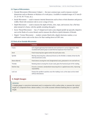3. Height Gauges DEFINITION A height gauge is a precision instrument used, in conjunction with a surface plate, to measure the vertical height of a component from a datum surface, or to scribe accurate reference/marking lines at a specified height.
• 9.
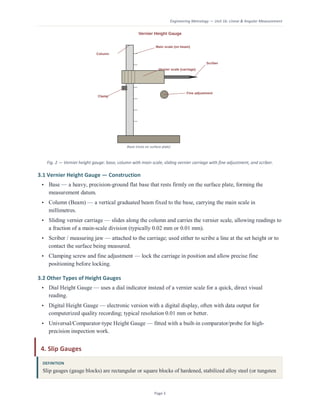
  Engineering Metrology —Unit 1b: Linear & Angular Measurement Page 3 Fig. 2 — Vernier height gauge: base, column with main scale, sliding vernier carriage with fine adjustment, and scriber. 3.1 Vernier Height Gauge — Construction • Base — a heavy, precision-ground flat base that rests firmly on the surface plate, forming the measurement datum. • Column (Beam) — a vertical graduated beam fixed to the base, carrying the main scale in millimetres. • Sliding vernier carriage — slides along the column and carries the vernier scale, allowing readings to a fraction of a main-scale division (typically 0.02 mm or 0.01 mm). • Scriber / measuring jaw — attached to the carriage; used either to scribe a line at the set height or to contact the surface being measured. • Clamping screw and fine adjustment — lock the carriage in position and allow precise fine positioning before locking. 3.2 Other Types of Height Gauges • Dial Height Gauge — uses a dial indicator instead of a vernier scale for a quick, direct visual reading. • Digital Height Gauge — electronic version with a digital display, often with data output for computerized quality recording; typical resolution 0.01 mm or better. • Universal/Comparator-type Height Gauge — fitted with a built-in comparator/probe for high- precision inspection work. 4. Slip Gauges DEFINITION Slip gauges (gauge blocks) are rectangular or square blocks of hardened, stabilized alloy steel (or tungsten
• 10.
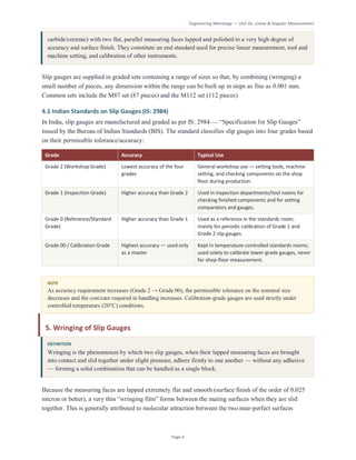
  Engineering Metrology —Unit 1b: Linear & Angular Measurement Page 4 carbide/ceramic) with two flat, parallel measuring faces lapped and polished to a very high degree of accuracy and surface finish. They constitute an end standard used for precise linear measurement, tool and machine setting, and calibration of other instruments. Slip gauges are supplied in graded sets containing a range of sizes so that, by combining (wringing) a small number of pieces, any dimension within the range can be built up in steps as fine as 0.001 mm. Common sets include the M87 set (87 pieces) and the M112 set (112 pieces). 4.1 Indian Standards on Slip Gauges (IS: 2984) In India, slip gauges are manufactured and graded as per IS: 2984 — “Specification for Slip Gauges” issued by the Bureau of Indian Standards (BIS). The standard classifies slip gauges into four grades based on their permissible tolerance/accuracy: Grade Accuracy Typical Use Grade 2 (Workshop Grade) Lowest accuracy of the four grades General workshop use — setting tools, machine setting, and checking components on the shop floor during production. Grade 1 (Inspection Grade) Higher accuracy than Grade 2 Used in inspection departments/tool rooms for checking finished components and for setting comparators and gauges. Grade 0 (Reference/Standard Grade) Higher accuracy than Grade 1 Used as a reference in the standards room, mainly for periodic calibration of Grade 1 and Grade 2 slip gauges. Grade 00 / Calibration Grade Highest accuracy — used only as a master Kept in temperature-controlled standards rooms; used solely to calibrate lower-grade gauges, never for shop-floor measurement. NOTE As accuracy requirement increases (Grade 2 → Grade 00), the permissible tolerance on the nominal size decreases and the cost/care required in handling increases. Calibration-grade gauges are used strictly under controlled temperature (20°C) conditions. 5. Wringing of Slip Gauges DEFINITION Wringing is the phenomenon by which two slip gauges, when their lapped measuring faces are brought into contact and slid together under slight pressure, adhere firmly to one another — without any adhesive — forming a solid combination that can be handled as a single block. Because the measuring faces are lapped extremely flat and smooth (surface finish of the order of 0.025 micron or better), a very thin “wringing film” forms between the mating surfaces when they are slid together. This is generally attributed to molecular attraction between the two near-perfect surfaces
• 11.
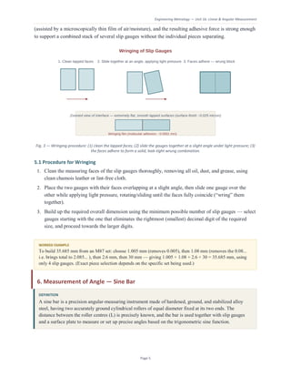
  Engineering Metrology —Unit 1b: Linear & Angular Measurement Page 5 (assisted by a microscopically thin film of air/moisture), and the resulting adhesive force is strong enough to support a combined stack of several slip gauges without the individual pieces separating. Fig. 3 — Wringing procedure: (1) clean the lapped faces; (2) slide the gauges together at a slight angle under light pressure; (3) the faces adhere to form a solid, leak-tight wrung combination. 5.1 Procedure for Wringing 1. Clean the measuring faces of the slip gauges thoroughly, removing all oil, dust, and grease, using clean chamois leather or lint-free cloth. 2. Place the two gauges with their faces overlapping at a slight angle, then slide one gauge over the other while applying light pressure, rotating/sliding until the faces fully coincide (“wring” them together). 3. Build up the required overall dimension using the minimum possible number of slip gauges — select gauges starting with the one that eliminates the rightmost (smallest) decimal digit of the required size, and proceed towards the larger digits. WORKED EXAMPLE To build 35.685 mm from an M87 set: choose 1.005 mm (removes 0.005), then 1.08 mm (removes the 0.08... i.e. brings total to 2.085... ), then 2.6 mm, then 30 mm — giving 1.005 + 1.08 + 2.6 + 30 = 35.685 mm, using only 4 slip gauges. (Exact piece selection depends on the specific set being used.) 6. Measurement of Angle — Sine Bar DEFINITION A sine bar is a precision angular-measuring instrument made of hardened, ground, and stabilized alloy steel, having two accurately ground cylindrical rollers of equal diameter fixed at its two ends. The distance between the roller centres (L) is precisely known, and the bar is used together with slip gauges and a surface plate to measure or set up precise angles based on the trigonometric sine function.
• 12.
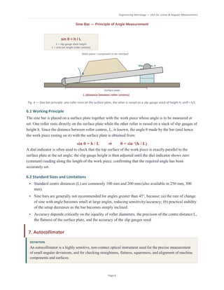
  Engineering Metrology —Unit 1b: Linear & Angular Measurement Page 6 Fig. 4 — Sine bar principle: one roller rests on the surface plate, the other is raised on a slip-gauge stack of height h; sinθ = h/L. 6.1 Working Principle The sine bar is placed on a surface plate together with the work piece whose angle is to be measured or set. One roller rests directly on the surface plate while the other roller is raised on a stack of slip gauges of height h. Since the distance between roller centres, L, is known, the angle θ made by the bar (and hence the work piece resting on it) with the surface plate is obtained from: sin θ = h / L ⇒ θ = sin⁻¹(h / L) A dial indicator is often used to check that the top surface of the work piece is exactly parallel to the surface plate at the set angle; the slip gauge height is then adjusted until the dial indicator shows zero (constant) reading along the length of the work piece, confirming that the required angle has been accurately set. 6.2 Standard Sizes and Limitations • Standard centre distances (L) are commonly 100 mm and 200 mm (also available in 250 mm, 300 mm). • Sine bars are generally not recommended for angles greater than 45°, because: (a) the rate of change of sine with angle becomes small at large angles, reducing sensitivity/accuracy; (b) practical stability of the setup decreases as the bar becomes steeply inclined. • Accuracy depends critically on the equality of roller diameters, the precision of the centre distance L, the flatness of the surface plate, and the accuracy of the slip gauges used. 7. Autocollimator DEFINITION An autocollimator is a highly sensitive, non-contact optical instrument used for the precise measurement of small angular deviations, and for checking straightness, flatness, squareness, and alignment of machine components and surfaces.
• 13.
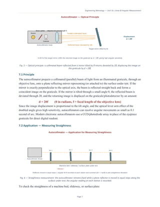
  Engineering Metrology —Unit 1b: Linear & Angular Measurement Page 7 Fig. 5 — Optical principle: a collimated beam reflected from a mirror tilted by θ returns deviated by 2θ, displacing the image on the graticule by d = 2θf. 7.1 Principle The autocollimator projects a collimated (parallel) beam of light from an illuminated graticule, through an objective lens, onto a plane reflecting mirror representing (or attached to) the surface under test. If the mirror is exactly perpendicular to the optical axis, the beam is reflected straight back and forms a coincident image on the graticule. If the mirror is tilted through a small angle θ, the reflected beam is deviated through 2θ, and the returning image is displaced on the graticule/photodetector by an amount: d = 2θf (θ in radians, f = focal length of the objective lens) Since the image displacement is proportional to the tilt angle, and the optical lever arm effect of the doubled angle gives high sensitivity, autocollimators can resolve angular movements as small as 0.1 second of arc. Modern electronic autocollimators use a CCD/photodiode array in place of the eyepiece graticule for direct digital readout. 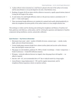7.2 Application — Measuring Straightness Fig. 6 — Straightness measurement: the autocollimator remains fixed while a plane reflector is moved in equal steps along the surface under test; the angular reading at each station is recorded. To check the straightness of a machine bed, slideway, or surface plate:
• 14.
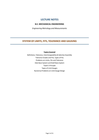
  Engineering Metrology —Unit 1b: Linear & Angular Measurement Page 8 4. A plane reflector mirror (mounted on a small base) is placed at the start of the surface to be tested, and the autocollimator is set up and aligned at one end, a fixed distance away. 5. Readings of angular tilt (θ) are taken with the reflector at successive, equally spaced stations (interval l) along the full length of the surface. 6. At each station, the small height difference relative to the previous station is calculated as Δh = l · tanθ ≈ l · θ (for small angles). 7. These incremental height differences are cumulatively summed (and usually plotted graphically) to obtain the straightness deviation profile of the surface relative to a true straight reference line. This technique is widely used for checking and certifying the straightness and flatness of machine tool beds, guideways and slideways, surface plates, and for verifying the squareness and alignment of machine components during installation, erection, and periodic calibration. Quick Revision — Key Points to Remember • Micrometer least count = pitch ÷ number of thimble divisions; common types — outside, inside, depth, and screw-thread micrometers. • Vernier height gauge measures height from a datum (surface plate) and can also scribe reference lines; dial and digital variants also exist. • Slip gauges are end standards, graded per IS: 2984 as Grade 2 (workshop) → Grade 1 (inspection) → Grade 0 (reference) → Grade 00/Calibration (master). • Wringing = molecular adhesion between two lapped, clean slip-gauge faces slid together — no adhesive required. • Sine bar: sinθ = h/L; not recommended above 45° due to reduced sensitivity at large angles. • Autocollimator: image displacement d = 2θf; used for angular measurement, and for straightness/flatness/squareness checks on machine surfaces.
• 15.
  Page 1 of15 LECTURE NOTES B.E. MECHANICAL ENGINEERING Engineering Metrology and Measurements SYSTEM OF LIMITS, FITS, TOLERANCE AND GAUGING Topics Covered Definitions, Tolerance, Interchangeability & Selective Assembly Tolerance Grades and Fits, Types of Fits Problems on Limits, Fits and Tolerance Hole Basis System and Shaft Basis System Taylor's Principle Types of Limit Gauges Numerical Problems on Limit Gauge Design
• 16.
  Page 2 of15 Table of Contents 1. Introduction.........................................................................................................................................3 2. Definitions and Terminology................................................................................................................3 3. Types of Tolerance...............................................................................................................................4 4. Interchangeability................................................................................................................................5 5. Selective Assembly...............................................................................................................................5 6. Tolerance Grades (IT Grades)...............................................................................................................6 7. Fits.......................................................................................................................................................7 8. Hole Basis and Shaft Basis Systems ......................................................................................................9 9. Taylor's Principle of Gauge Design......................................................................................................10 10. Types of Limit Gauges ......................................................................................................................12 11. Numerical Problems.........................................................................................................................13 12. Summary of Key Formulas................................................................................................................14
• 17.
  Page 3 of15 1. Introduction In any manufacturing process, it is impossible to produce a component to an exact, perfect size due to inherent inaccuracies of machine tools, tool wear, deflection, operator skill and measuring errors. Every dimension produced therefore varies slightly from the intended (basic) size. If components are to be interchangeable — that is, if any one component can be assembled with any mating component without individual fitting or selection — this variation must be controlled within specified boundaries. The System of Limits, Fits and Tolerances is the standardised method (as per IS 919 in India, based on ISO 286) of specifying these permissible size variations for holes and shafts so that a desired relationship — clearance, interference or transition — is guaranteed on assembly. Gauging is the practical means by which these limits are verified on the shop floor using limit gauges instead of precision measuring instruments, making inspection quick and economical for mass production. 2. Definitions and Terminology Fig. 1 Terminology of Limits and Fits (Zero Line Diagram) 2.1 Basic Terms Nominal Size: The size of a part used for general identification, usually expressed in whole numbers, e.g. ‘50 mm’. It is simply a convenient round number by which the dimension is referred to. Basic Size (Basic Dimension): The size arrived at purely from design/strength calculations, to which all limits of size are applied to arrive at the final dimensions. The basic size of the hole and the shaft of a mating pair is the same. Actual Size: The size of a component as obtained after manufacture, found by actual measurement.
• 18.
  Page 4 of15 Limits of Size: The two extreme permissible sizes for a dimension of a part, between which the actual size should lie. The larger of the two is the Maximum Limit of Size, and the smaller is the Minimum Limit of Size. Zero Line: A straight line corresponding to the basic size, drawn horizontally, with respect to which deviations are graphically represented. Positive deviations are shown above the zero line and negative deviations below it (by convention). Deviation: The algebraic difference between a size (actual, maximum or minimum) and the corresponding basic size. Upper Deviation: The algebraic difference between the maximum limit of size and the basic size. Denoted ES for a hole (Écart Supérieur) and es for a shaft. Lower Deviation: The algebraic difference between the minimum limit of size and the basic size. Denoted EI for a hole (Écart Inférieur) and ei for a shaft. Fundamental Deviation: Of the two deviations, the one nearer to the zero line, used to fix the position of the tolerance zone relative to the basic size. It is represented by a letter — capital letters (A–ZC) for holes and small letters (a–zc) for shafts. Tolerance: The difference between the maximum limit of size and the minimum limit of size of a part. It is always an absolute (unsigned) value. Tolerance = High Limit − Low Limit. Tolerance Zone: The zone between the two limits of size, defined by the magnitude of the tolerance and its position with respect to the zero line. Allowance: The intentional difference between the low limit of the hole and the high limit of the shaft in a hole-and-shaft assembly. It represents the tightest possible fit and may be positive (clearance) or negative (interference). 3. Types of Tolerance Fig. 2 Unilateral and Bilateral Tolerance 3.1 Unilateral Tolerance When the tolerance (variation) is allowed only on one side of the basic size — either entirely above it or entirely below it — it is called unilateral tolerance. Example: 25.00 +0.04/+0.00 mm.
• 19.
  Page 5 of15 Unilateral tolerancing is preferred in interchangeable manufacture because it allows the basic size to also represent one of the limits (usually the Maximum Metal Limit), which simplifies the design of limit gauges — the GO gauge can be made to the basic size. 3.2 Bilateral Tolerance When the tolerance is distributed on both sides of the basic size, i.e. partly positive and partly negative, it is called bilateral tolerance. Example: 25.00 +0.02/−0.02 mm. Bilateral tolerancing is generally used in general engineering practice where machining is done directly to the basic size shown on the drawing, without necessarily using limit gauges. 4. Interchangeability Definition: Interchangeability is the property that permits the replacement of one part by another similar part manufactured to the same specification, without any additional fitting, and without affecting the functioning of the assembly. Interchangeable manufacture is the backbone of mass production. It allows components to be manufactured in bulk at different times, in different factories, or even by different manufacturers, and yet be assembled and used as spare parts without hand-fitting. 4.1 Types of Interchangeability • Universal Interchangeability: Mating parts manufactured at different locations (different machines, factories, or firms) can be assembled and replaced without selective fitting. This demands strict adherence to standardised limits and fits (e.g. IS 919 / ISO 286). • Local Interchangeability: Mating parts are manufactured and used for replacement within one factory only, using the same set of machines and gauges. The tolerances used may not conform to a national/international standard. 4.2 Conditions for Interchangeable Manufacture • The dimensions of mating parts must be controlled by limits based on a standardised system of limits and fits. • Suitable fits (clearance, transition or interference) must be selected to suit the functional requirement of the assembly. • Parts must be checked using limit gauges designed as per Taylor's Principle rather than by precision measurement of every dimension. 5. Selective Assembly In certain high-precision assemblies (e.g. ball and roller bearings, piston-pin-bush assemblies, precision gauges), the functional tolerance required is extremely small — so small that producing every component to that tolerance by normal interchangeable manufacture would be technically difficult and prohibitively expensive.
• 20.
  Page 6 of15 Principle: Components are manufactured to a comparatively wider, economical tolerance. After manufacture, each finished part is measured and sorted (segregated) into a number of groups based on its actual size, using a graduated gauge. Parts are then assembled only from matching groups — for example, the largest holes are assembled only with the largest shafts of the matching group, giving the equivalent of a very fine tolerance fit. 5.1 Advantages • Achieves very high precision of fit that would otherwise be uneconomical to manufacture directly. • Manufacturing cost is reduced since components are produced to a wider, easily achievable tolerance. • Rejection rate is minimised, since a part that lies outside the desired tight limits is simply placed in a different matching group instead of being scrapped. 5.2 Limitation Selective assembly sacrifices universal interchangeability — a part from one size-group cannot be freely interchanged with a part from another group, and hence it is generally restricted to local/plant-level interchangeability. 6. Tolerance Grades (IT Grades) The magnitude of tolerance (the width of the tolerance zone) is standardised into 18 grades called Fundamental Tolerance grades or International Tolerance (IT) grades, numbered IT01, IT0, IT1, IT2 … up to IT16 (extended to IT18 in later revisions of ISO 286 / IS 919). The tolerance value increases from IT01 (finest) to IT16 (coarsest), while the letter symbol (fundamental deviation) fixes the position of the zone relative to the zero line. 6.1 Standard Tolerance Unit For sizes up to 500 mm, the standard tolerance unit ‘i’ (in microns) used to compute the numerical value of every IT grade is given by: i = 0.45 × D¹ᶠ³ + 0.001 D (microns, D in mm) where D is the geometric mean diameter of the size range under consideration, D = √(D₁ × D₂), D₁ and D₂ being the lower and upper values of the size range (sizes are grouped into standard steps such as 1–3, 3– 6, 6–10, 10–18, 18–30, 30–50, 50–80 mm, etc., to keep the tolerance calculation manageable). The tolerance for a given IT grade is obtained by multiplying ‘i’ by a standard multiplying factor, as listed below: IT Grade Multiplier IT Grade Multiplier IT Grade Multiplier IT5 7i IT9 40i IT13 250i IT6 10i IT10 64i IT14 400i IT7 16i IT11 100i IT15 640i IT8 25i IT12 160i IT16 1000i
• 21.
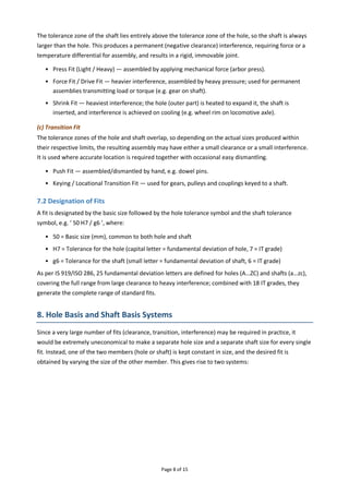
  Page 7 of15 6.2 Application of IT Grades IT Grade Range Typical Application IT01 – IT4 Gauge blocks, precision gauges, reference standards (lapping, honing, fine grinding) IT5 – IT7 Precision machining — grinding, fine turning/boring; used for fits (mating hole/shaft) IT8 – IT11 General engineering manufacture — turning, milling, drilling, boring IT12 – IT16 Rough machining, sheet-metal work, press work, casting/forging 7. Fits Definition: A fit is the relationship that exists between two mating parts — a hole and a shaft — with respect to the difference in their sizes, before assembly, which governs the amount of clearance or interference obtained when they are assembled together. 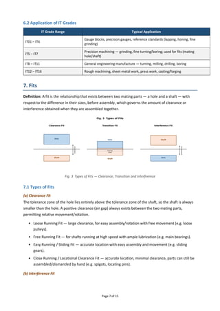Fig. 3 Types of Fits — Clearance, Transition and Interference 7.1 Types of Fits (a) Clearance Fit The tolerance zone of the hole lies entirely above the tolerance zone of the shaft, so the shaft is always smaller than the hole. A positive clearance (air gap) always exists between the two mating parts, permitting relative movement/rotation. • Loose Running Fit — large clearance, for easy assembly/rotation with free movement (e.g. loose pulleys). • Free Running Fit — for shafts running at high speed with ample lubrication (e.g. main bearings). • Easy Running / Sliding Fit — accurate location with easy assembly and movement (e.g. sliding gears). • Close Running / Locational Clearance Fit — accurate location, minimal clearance, parts can still be assembled/dismantled by hand (e.g. spigots, locating pins). (b) Interference Fit
• 22.
  Page 8 of15 The tolerance zone of the shaft lies entirely above the tolerance zone of the hole, so the shaft is always larger than the hole. This produces a permanent (negative clearance) interference, requiring force or a temperature differential for assembly, and results in a rigid, immovable joint. • Press Fit (Light / Heavy) — assembled by applying mechanical force (arbor press). • Force Fit / Drive Fit — heavier interference, assembled by heavy pressure; used for permanent assemblies transmitting load or torque (e.g. gear on shaft). • Shrink Fit — heaviest interference; the hole (outer part) is heated to expand it, the shaft is inserted, and interference is achieved on cooling (e.g. wheel rim on locomotive axle). (c) Transition Fit The tolerance zones of the hole and shaft overlap, so depending on the actual sizes produced within their respective limits, the resulting assembly may have either a small clearance or a small interference. It is used where accurate location is required together with occasional easy dismantling. • Push Fit — assembled/dismantled by hand, e.g. dowel pins. • Keying / Locational Transition Fit — used for gears, pulleys and couplings keyed to a shaft. 7.2 Designation of Fits A fit is designated by the basic size followed by the hole tolerance symbol and the shaft tolerance symbol, e.g. ‘ 50 H7 / g6 ’, where: • 50 = Basic size (mm), common to both hole and shaft • H7 = Tolerance for the hole (capital letter = fundamental deviation of hole, 7 = IT grade) • g6 = Tolerance for the shaft (small letter = fundamental deviation of shaft, 6 = IT grade) As per IS 919/ISO 286, 25 fundamental deviation letters are defined for holes (A…ZC) and shafts (a…zc), covering the full range from large clearance to heavy interference; combined with 18 IT grades, they generate the complete range of standard fits. 8. Hole Basis and Shaft Basis Systems Since a very large number of fits (clearance, transition, interference) may be required in practice, it would be extremely uneconomical to make a separate hole size and a separate shaft size for every single fit. Instead, one of the two members (hole or shaft) is kept constant in size, and the desired fit is obtained by varying the size of the other member. This gives rise to two systems:
• 23.
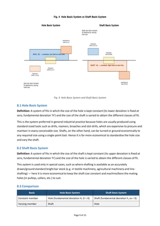
  Page 9 of15 Fig. 4 Hole Basis System and Shaft Basis System 8.1 Hole Basis System Definition: A system of fits in which the size of the hole is kept constant (its lower deviation is fixed at zero, fundamental deviation ‘H’) and the size of the shaft is varied to obtain the different classes of fit. This is the system preferred in general industrial practice because holes are usually produced using standard-sized tools such as drills, reamers, broaches and slot-drills, which are expensive to procure and maintain in every conceivable size. Shafts, on the other hand, can be turned or ground economically to any required size using a single-point tool. Hence it is far more economical to standardise the hole size and vary the shaft. 8.2 Shaft Basis System Definition: A system of fits in which the size of the shaft is kept constant (its upper deviation is fixed at zero, fundamental deviation ‘h’) and the size of the hole is varied to obtain the different classes of fit. This system is used only in special cases, such as where shafting is available as an accurately drawn/ground standard bright bar stock (e.g. in textile machinery, agricultural machinery and line- shafting) — here it is more economical to keep the shaft size constant and machine/bore the mating holes (in pulleys, collars, etc.) to suit. 8.3 Comparison Basis Hole Basis System Shaft Basis System Constant member Hole (fundamental deviation H, EI = 0) Shaft (fundamental deviation h, es = 0) Varying member Shaft Hole
• 24.
  Page 10 of15 Basis Hole Basis System Shaft Basis System Tooling economy Uses standard drills/reamers for holes; shafts turned to size Uses standard ground shaft stock; holes bored to size Preferred use General engineering industry (widely preferred) Textile/agricultural machinery, line shafting 9. Taylor's Principle of Gauge Design Taylor's Principle (also called the Principle of Gauging) lays down the fundamental rule for designing GO and NOGO limit gauges so that they correctly accept all good parts and reject all defective parts, checking both size and form errors. 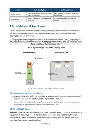“GO gauge should be designed to check the Maximum Metal Limit (MML), inspecting all related dimensions simultaneously; the NOGO gauge should check only the Minimum Metal Limit (LML), one dimension at a time.” Fig. 5 Taylor's Principle — GO and NO GO Gauge Design 9.1 Maximum and Minimum Metal Limits • Maximum Metal Limit (MML): the limit of size at which the part contains the maximum amount of material — the Low Limit for a hole, and the High Limit for a shaft. • Minimum Metal Limit (LML): the limit of size at which the part contains the minimum amount of material — the High Limit for a hole, and the Low Limit for a shaft. 9.2 GO and NOGO Gauges GO Gauge: Checks the Maximum Metal Limit. It is made a ‘full form’ gauge — as long as the full length of engagement of the mating part — so that it checks the size at every cross-section along the length simultaneously, thereby also revealing errors of form such as ovality, taper and bending. A good part must allow the GO gauge to pass/enter freely.
• 25.
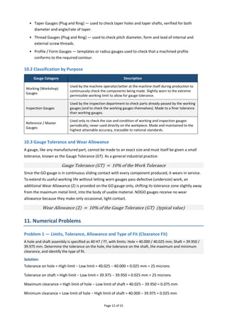
  Page 11 of15 NOGO Gauge: Checks the Minimum Metal Limit. It is deliberately made short, checking the size only at one cross-section (or a few isolated points), because it is only required to check size, not form, at the tightest limit. A good part must NOT allow the NOGO gauge to pass/enter. 9.3 Reason for the Rule The GO gauge is in continuous, sliding contact with every part produced, over its full working length, and therefore wears out faster; keeping it full-form ensures that as long as it is within its wear-allowance tolerance it still correctly enforces both size and geometric form. The NOGO gauge only makes light contact at isolated points on a small percentage of parts (those close to the limit), so wear is negligible and a short/point-contact form is adequate and economical. Note: For very large-diameter plug gauges, a full-form GO gauge becomes too heavy and costly to manufacture and handle; in such cases the principle is knowingly relaxed and other means (progressive or segmental gauges) are used, supplemented by additional inspection for form errors. 10. Types of Limit Gauges A limit gauge is a precision inspection tool made to the limiting (GO/NOGO) sizes of a dimension. Unlike a measuring instrument, it does not indicate the actual size of a part — it only indicates whether the part lies within the specified limits (Accept) or outside them (Reject), making inspection extremely rapid, which is essential in mass production. 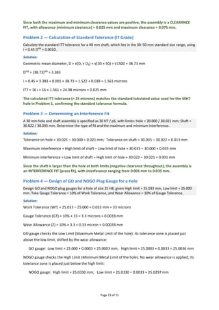Fig. 6 Common Types of Limit Gauges 10.1 Classification by Form • Plug Gauge — a cylindrical gauge used to check the size of a hole (bore); usually double-ended with a GO end (longer, checks the low/MML limit) and a NOGO end (shorter, checks the high/LML limit). • Ring Gauge — an internally ground/lapped ring used to check the size of a shaft (external diameter); separate GO and NOGO rings are used, usually distinguished by an annular groove on the NOGO ring. • Snap Gauge / Gap Gauge — a caliper-type gauge with fixed or adjustable anvils, used to check shaft/external dimensions; portable and does not need to be passed over the full length of the shaft, so it is convenient for large or long components.
• 26.
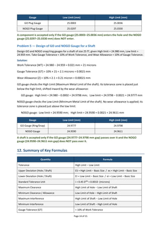
  Page 12 of15 • Taper Gauges (Plug and Ring) — used to check taper holes and taper shafts, verified for both diameter and angle/rate of taper. • Thread Gauges (Plug and Ring) — used to check pitch diameter, form and lead of internal and external screw threads. • Profile / Form Gauges — templates or radius gauges used to check that a machined profile conforms to the required contour. 10.2 Classification by Purpose Gauge Category Description Working (Workshop) Gauges Used by the machine operator/setter at the machine itself during production to continuously check the components being made. Slightly worn to the extreme permissible working limit to allow for gauge tolerance. Inspection Gauges Used by the inspection department to check parts already passed by the working gauges (and to check the working gauges themselves). Made to a finer tolerance than working gauges. Reference / Master Gauges Used only to check the size and condition of working and inspection gauges periodically; never used directly on the workpiece. Made and maintained to the highest attainable accuracy, traceable to national standards. 10.3 Gauge Tolerance and Wear Allowance A gauge, like any manufactured part, cannot be made to an exact size and must itself be given a small tolerance, known as the Gauge Tolerance (GT). As a general industrial practice: Gauge Tolerance (GT) = 10% of the Work Tolerance Since the GO gauge is in continuous sliding contact with every component produced, it wears in service. To extend its useful working life without letting worn gauges pass defective (undersize) work, an additional Wear Allowance (Z) is provided on the GO gauge only, shifting its tolerance zone slightly away from the maximum metal limit, into the body of usable material. NOGO gauges receive no wear allowance because they make only occasional, light contact. Wear Allowance (Z) = 10% of the Gauge Tolerance (GT) (typical value) 11. Numerical Problems Problem 1 — Limits, Tolerance, Allowance and Type of Fit (Clearance Fit) A hole and shaft assembly is specified as 40 H7 / f7, with limits: Hole = 40.000 / 40.025 mm; Shaft = 39.950 / 39.975 mm. Determine the tolerance on the hole, the tolerance on the shaft, the maximum and minimum clearance, and identify the type of fit. Solution: Tolerance on hole = High limit − Low limit = 40.025 − 40.000 = 0.025 mm = 25 microns Tolerance on shaft = High limit − Low limit = 39.975 − 39.950 = 0.025 mm = 25 microns Maximum clearance = High limit of hole − Low limit of shaft = 40.025 − 39.950 = 0.075 mm Minimum clearance = Low limit of hole − High limit of shaft = 40.000 − 39.975 = 0.025 mm
• 27.
  Page 13 of15 Since both the maximum and minimum clearance values are positive, the assembly is a CLEARANCE FIT, with allowance (minimum clearance) = 0.025 mm and maximum clearance = 0.075 mm. Problem 2 — Calculation of Standard Tolerance (IT Grade) Calculate the standard IT7 tolerance for a 40 mm shaft, which lies in the 30–50 mm standard size range, using i = 0.45 D¹ᶠ³ + 0.001D. Solution: Geometric mean diameter, D = √(D₁ × D₂) = √(30 × 50) = √1500 = 38.73 mm D¹ᶠ³ = (38.73)¹ᶠ³ = 3.383 i = 0.45 × 3.383 + 0.001 × 38.73 = 1.522 + 0.039 = 1.561 microns IT7 = 16 i = 16 × 1.561 = 24.98 microns ≈ 0.025 mm The calculated IT7 tolerance (≈ 25 microns) matches the standard tabulated value used for the 40H7 hole in Problem 1, confirming the standard tolerance formula. Problem 3 — Determining an Interference Fit A 30 mm hole and shaft assembly is specified as 30 H7 / p6, with limits: Hole = 30.000 / 30.021 mm; Shaft = 30.022 / 30.035 mm. Determine the type of fit and the maximum and minimum interference. Solution: Tolerance on hole = 30.021 − 30.000 = 0.021 mm; Tolerance on shaft = 30.035 − 30.022 = 0.013 mm Maximum interference = High limit of shaft − Low limit of hole = 30.035 − 30.000 = 0.035 mm Minimum interference = Low limit of shaft − High limit of hole = 30.022 − 30.021 = 0.001 mm Since the shaft is larger than the hole at both limits (negative clearance throughout), the assembly is an INTERFERENCE FIT (press fit), with interference ranging from 0.001 mm to 0.035 mm. Problem 4 — Design of GO and NOGO Plug Gauge for a Hole Design GO and NOGO plug gauges for a hole of size 25 H8, given High limit = 25.033 mm, Low limit = 25.000 mm. Take Gauge Tolerance = 10% of Work Tolerance, and Wear Allowance = 10% of Gauge Tolerance. Solution: Work Tolerance (WT) = 25.033 − 25.000 = 0.033 mm = 33 microns Gauge Tolerance (GT) = 10% × 33 = 3.3 microns = 0.0033 mm Wear Allowance (Z) = 10% × 3.3 = 0.33 micron = 0.00033 mm GO gauge checks the Low Limit (Maximum Metal Limit of the hole). Its tolerance zone is placed just above the low limit, shifted by the wear allowance: GO gauge: Low limit = 25.000 + 0.0003 = 25.0003 mm; High limit = 25.0003 + 0.0033 = 25.0036 mm NOGO gauge checks the High Limit (Minimum Metal Limit of the hole). No wear allowance is applied; its tolerance zone is placed just below the high limit: NOGO gauge: High limit = 25.0330 mm; Low limit = 25.0330 − 0.0033 = 25.0297 mm
• 28.
  Page 14 of15 Gauge Low Limit (mm) High Limit (mm) GO Plug Gauge 25.0003 25.0036 NOGO Plug Gauge 25.0297 25.0330 A component is accepted only if the GO gauge (25.0003–25.0036 mm) enters the hole and the NOGO gauge (25.0297–25.0330 mm) does NOT enter. Problem 5 — Design of GO and NOGO Gauge for a Shaft Design GO and NOGO snap/ring gauges for a shaft of size 25 f7, given High limit = 24.980 mm, Low limit = 24.959 mm. Take Gauge Tolerance = 10% of Work Tolerance, and Wear Allowance = 10% of Gauge Tolerance. Solution: Work Tolerance (WT) = 24.980 − 24.959 = 0.021 mm = 21 microns Gauge Tolerance (GT) = 10% × 21 = 2.1 microns = 0.0021 mm Wear Allowance (Z) = 10% × 2.1 = 0.21 micron = 0.00021 mm GO gauge checks the High Limit (Maximum Metal Limit of the shaft). Its tolerance zone is placed just below the high limit, shifted inward by the wear allowance: GO gauge: High limit = 24.980 − 0.0002 = 24.9798 mm; Low limit = 24.9798 − 0.0021 = 24.9777 mm NOGO gauge checks the Low Limit (Minimum Metal Limit of the shaft). No wear allowance is applied; its tolerance zone is placed just above the low limit: NOGO gauge: Low limit = 24.9590 mm; High limit = 24.9590 + 0.0021 = 24.9611 mm Gauge Low Limit (mm) High Limit (mm) GO Gauge (Ring/Snap) 24.9777 24.9798 NOGO Gauge 24.9590 24.9611 A shaft is accepted only if the GO gauge (24.9777–24.9798 mm gap) passes over it and the NOGO gauge (24.9590–24.9611 mm gap) does NOT pass over it. 12. Summary of Key Formulas Quantity Formula Tolerance High Limit − Low Limit Upper Deviation (Hole / Shaft) ES = High Limit − Basic Size / es = High Limit − Basic Size Lower Deviation (Hole / Shaft) EI = Low Limit − Basic Size / ei = Low Limit − Basic Size Standard Tolerance Unit i = 0.45 D¹ᶠ³ + 0.001D (microns) Maximum Clearance High Limit of Hole − Low Limit of Shaft Minimum Clearance / Allowance Low Limit of Hole − High Limit of Shaft Maximum Interference High Limit of Shaft − Low Limit of Hole Minimum Interference Low Limit of Shaft − High Limit of Hole Gauge Tolerance (GT) ≈ 10% of Work Tolerance
• 29.
  Page 15 of15 Quantity Formula Wear Allowance (Z) ≈ 10% of Gauge Tolerance