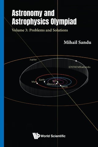
Comprehensive Astronomy and Astrophysics Olympiad Problems and Solutions Volume 3
Advanced problems and solutions in astronomy and astrophysics for Olympiad preparation, covering celestial mechanics, star systems, and space travel physics.
This page intentionallyleft blank
This page intentionally left blank
4.
Astronomy and
Astrophysics Olympiad
Volume3: Problems and Solutions
Mihail Sandu
Romanian Physics Olympiad Committee, Romania
World Scientific
NEW JERSEY • LONDON • SINGAPORE • BEIJING • SHANGHAI • HONG KONG • TAIPEI • CHENNAI • TOKYO
Foreword
Astronomy and Astrophysicsare among the oldest sciences, yet they
continue to undergo rapid development. Over time, the focus has
shifted from simple observations of celestial motions to detailed
investigations of galaxies, black holes and the cosmic microwave
background. Today, progress in these fields is shaped by powerful
telescopes, large-scale surveys, and theoretical models that push the
limits of our current knowledge.
Such progress depends not only on professional research but also
on the cultivation of new generations of scientists. Competitions
like the Astronomy Olympiad and the Astronomy and Astrophysics
Olympiad play an important role in this process. By challenging
high school students to engage with advanced concepts and problem-
solving techniques, these events help develop the critical skills and
curiosity essential for a career in science.
Despite their educational value, there remains a lack of com-
prehensive resources tailored specifically to these Olympiads. The
present collection of three volumes, containing original problems
crafted by Professor Mihail Sandu, addresses this need in an out-
standing manner, offering students and teachers alike a wide range
of tools critically needed for preparing for such competitions.
Professor Sandu is a highly respected educator with decades of
experience at both high school and university levels. His contribu-
tions to academic competitions are remarkable. Among other achieve-
ments, he prepared all theory problems for the 2014 International
Olympiad on Astronomy and Astrophysics, as well as all practical
v
7.
vi Astronomy andAstrophysics Olympiad - Volume 3
test problems for the 2019 International Astronomy Olympiad, both
held in Romania. More recently, he played a key role in the first
Junior International Olympiad on Astronomy and Astrophysics in
2022. He has published nearly 100 books in Romanian and English,
including textbooks and problem collections in Physics and Astron-
omy that have guided generations of students.
I have had the privilege of knowing Professor Sandu personally.
His dedication, clarity of thought, and genuine enthusiasm for teach-
ing are evident both in his presence at competitions and in his writ-
ing. Over more than five decades, he has supported and inspired
countless students, exemplifying a rare commitment to education and
mentorship. I am confident that the present collection will prove to
be an invaluable resource for students preparing for Olympiads, and
that it will continue to inspire future generations of astronomers and
astrophysicists.
Andrei Constantin
Royal Society Dorothy Hodgkin Fellow,
Department of Physics, University of Oxford,
and Physics & Mathematics Tutor
at Mansfield College Oxford
8.
Contents
Foreword v
Problem 1.A Spaceship to Alpha Centauri 1
Problem 2. Asteroid 2010GD37 13
Problem 3. A Galaxy of Stars Identical
to Our Sun! 31
Problem 4. Two Astronomical Observatories
on an Island 37
Problem 5. Moons of Jupiter 73
Problem 6. A Comet Around the Sun 79
Problem 7. Visible Circumpolar Stars 81
Problem 8. Cepheid Period 89
Problem 9. Satellites with Orbits in
Perpendicular Planes 95
Problem 10. Solar City Tower 103
Problem 11. Temperature of Interstellar Space 113
vii
9.
viii Astronomy andAstrophysics Olympiad - Volume 3
Problem 12. Time Integral Mean Values and the
Virial Theorem 119
Problem 13. The Horizontal Diurnal Parallax of
a Star, Accurately Determined 133
Problem 14. Geostationary Satellite 153
Problem 15. Limits and Astronomical Spheres 159
Problem 16. Sunrise 169
Problem 17. Atmospheric Extinction 175
Problem 18. Geostationary Satellite in the
Plane of the Equator 185
Problem 19. Special Maneuvers of a
Geostationary Satellite 193
Problem 20. Precession of the World Axis 203
Problem 21. The Magnitudes of Stars 213
Problem 22. Bielliptic Gravitational Transfer 219
Problem 23. Photograph of Jupiter 223
Problem 24. The Mass Function of a Visual
Binary Star System 229
Problem 25. Length of a Day on Mars 235
Problem 26. The Temperature on the Surface
of the Sun 241
Problem 27. The Proper Motions of the Stars 245
Problem 28. The Orbits of the Planets 259
Problem 29. The Apparent Magnitude of the Sun 271
Problem 30. Altair and the Sun 277
10.
Contents ix
Problem 31.The Radii of Curvature of the
Moon’s Trajectory 289
Problem 32. Magnitudes of Stellar Systems 297
Problem 33. Visible Star? 301
Problem 34. The Meeting of the Stars 305
Problem 35. Law of Gravitational Attraction 311
Problem 36. Radial Velocities of Stars 315
Problem 37. Bombarding a Very Dangerous
Asteroid! 331
Problem 38. Virial Theorem 355
Problem 39. The Gravitational Potential
Energy of a Spherical Cluster 363
Problem 40. Jeans Mass 371
Problem 41. Free Fall Timescale 375
Problem 42. 85 Pegasi A and B 379
Problem 43. Convergent Proper Motions 387
Problem 44. From Romania . . . to the
Antipode! A Ballistic Projectile
Messenger 405
Problem 45. Ice Particle 421
Other Books by Mihail Sandu 435
11.
This page intentionallyleft blank
This page intentionally left blank
12.
Problem 1
A Spaceshipto Alpha Centauri
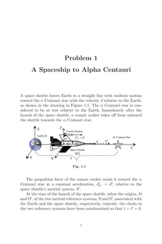
A space shuttle leaves Earth in a straight line with uniform motion
toward the α Centauri star with the velocity
u relative to the Earth,
as shown in the drawing in Figure 1.1. The α Centauri star is con-
sidered to be at rest relative to the Earth. Immediately after the
launch of the space shuttle, a cosmic rocket takes off from onboard
the shuttle towards the α Centauri star.
Fig. 1.1
The propulsion force of the cosmic rocket sends it toward the α
Centauri star at a constant acceleration,
a
Y =
a, relative to the
space shuttle’s inertial system, S.
At the time of the launch of the space shuttle, when the origins, O
and O, of the two inertial reference systems, S and S, associated with
the Earth and the space shuttle, respectively, coincide, the clocks in
the two reference systems have been synchronized so that t = t = 0.
1
13.
2 Astronomy andAstrophysics Olympiad - Volume 3
The cosmic rocket takes off from the space shuttle from the point
corresponding to the origin of the inertial system associated with the
space shuttle. The speed of light in a vacuum is c.
a) Establish the relationship between the acceleration of the cosmic
rocket in relation to the Earth, aY = a, and the speed of the
cosmic rocket in relation to the Earth, vY = v.
b) Establish the speed law of the cosmic rocket in relation to the
Earth, vY(t) = v(t).
c) Establish the law of acceleration of the cosmic rocket in relation
to the Earth, aY(t) = a(t).
d) Establish the law of the position coordinate of the cosmic rocket
in relation to the Earth, y(t). It is known that:
A + B · x
C + D · x
· dx =
1
D
B · x +
Δ
D
· ln |C + D · x|
;
Δ = AD − BC.
e) Determine the distance between the Earth and the α Centauri
star, Y , if the duration of the cosmic rocket’s travel between the
Earth and the α Centauri Star, relative to the observer on Earth,
is T.
f) Determine the speed of the cosmic rocket in relation to the Earth
at the time of its arrival at the α Centauri star.
g) Determine the duration of the movement of the cosmic rocket
between the Earth and the α Centauri star, timed by the observer
O on the space shuttle, T, as well as the distance traveled by the
cosmic rocket in relation to the observer O on the space shuttle
from the moment the rocket took off from the space shuttle until
its arrival at the α Centauri star, Y .
h) Particularize the results from parts b, c, and d for the case u c,
knowing that:
ln(1 + x) ≈ x −
1
2
x2
, if x 1.
Solution
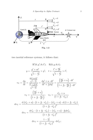
a) According to the notation in Figure 1.2, which corresponds to a
certain moment in the evolution of the cosmic rocket framed by the
14.
A Spaceship toAlpha Centauri 3
Fig. 1.2
two inertial reference systems, it follows that:
R
(0, y
, 0; t
); R(0, y, 0; t);
y =
y + ut
1 − u2
c2
y
; t =
t + uy
c2
1 − u2
c2
t
;
vY =
dy
dt
=
dy
+u·dt
1− u2
c2
dt
+ u
c2 dy
1− u2
c2
=
dy
+ u · dt
dt
+ u
c2 dy =
dy
dt + u
· dt
1 + u
c2 · dy
dt
· dt
;
vY =
dy
dt + u
1 + u
c2 · dy
dt
; vY =
v
Y + u
1 + u
c2 · v
Y
;
dvY =
d
v
Y + u ·
1 + u
c2 · v
Y −
v
Y + u · d
1 + u
c2 · v
Y
1 + u
c2 · v
Y
2 ;
dvY =
dv
Y ·
1 + u
c2 · v
Y −
v
Y + u · u
c2 dv
Y
1 + u
c2 · v
Y
2 ;
dvY =
1 − u2
c2
1 + u
c2 · v
Y
2 · dv
Y ;
15.
4 Astronomy andAstrophysics Olympiad - Volume 3
t =
t + uy
c2
1 − u2
c2
;
dt =
dt
+ u
c2 · dy
1 − u2
c2
=
1 + u
c2 · dy
dt
1 − u2
c2
· dt
;
dt =
1 + u
c2 · v
Y
1 − u2
c2
· dt
;
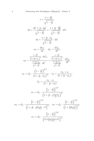
aY =
dvY
dt
; a
Y =
dv
Y
dt ;
aY =
1− u2
c2
1+ u
c2 ·v
Y
2 · dv
Y
1+ u
c2 ·v
Y
1− u2
c2
· dt
=
1− u2
c2
1+ u
c2 ·v
Y
2
1+ u
c2 ·v
Y
1− u2
c2
·
dv
Y
dt ;
aY = a
Y ·
1 − u2
c2
3/2
1 + u
c2 · v
Y
3 ; vY =
v
Y + u
1 + u
c2 · v
Y
;
v
Y =
vY − u
1 − u
c2 · vY
;
aY = a
Y ·
1 − u2
c2
3/2
1 + u
c2 · vY−u
1− u
c2 ·vY
3 ;
aY = a
Y ·
1 − u2
c2
3/2
1 + u
c2 · vY−u
c2−uvY
· c2
3 ; aY = a
Y ·
1 − u2
c2
3/2
1 + uvY−u2
c2−uvY
3 ;
aY = a
Y ·
1 − u2
c2
3/2
c2−uvY+uvY−u2
c2−uvY
3 ;
16.
A Spaceship toAlpha Centauri 5
aY = a
Y ·
1 − u2
c2
3/2
c2−u2
c2−uvY
3 ; aY = a
Y ·
1 − u2
c2
3/2
1− u2
c2
1−
uvY
c2
3 ;
aY = a
Y ·
1 − uvY
c2
3
1 − u2
c2
3/2
;
a
Y = a
; aY = a; vY = v; a = a
·
1 − uv
c2
3
1 − u2
c2
3/2
.
b)
vY =
u + v
Y
1 + u
c2 · v
Y
;
v
Y = a
Y · t
;
vY =
u + a
Y t
1 + u
c2 · a
Y t
;
t =
t + uy
c2
1 − u2
c2
t
; t
=
t − uy
c2
1 − u2
c2
t; y = ut;
t
=
t − u
c2 ut
1 − u2
c2
=
t
1 − u2
c2
1 − u2
c2
;
t
= t · 1 −
u2
c2
;
vY =
u + a
Y t
1 + u
c2 · a
Y t
;
vY =
u + a
Y ·
1 − u2
c2 · t
1 + u
c2 · a
Y ·
1 − u2
c2 · t
= vY(t); a
Y = a
; vY = v;
vY =
u + a
Y ·
1 − u2
c2 · t
1 + u
c2 · a
Y ·
1 − u2
c2 · t
= vY(t).
17.
6 Astronomy andAstrophysics Olympiad - Volume 3
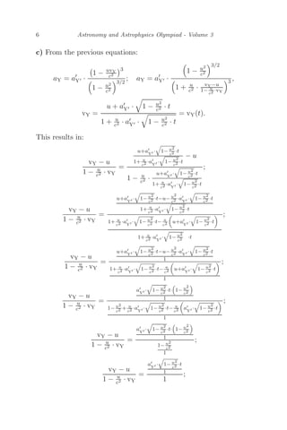
c) From the previous equations:
aY = a
Y ·
1 − uvY
c2
3
1 − u2
c2
3/2
; aY = a
Y ·
1 − u2
c2
3/2
1 + u
c2 · vY−u
1− u
c2 ·vY
3 ,
vY =
u + a
Y ·
1 − u2
c2 · t
1 + u
c2 · a
Y ·
1 − u2
c2 · t
= vY(t).
This results in:
vY − u
1 − u
c2 · vY
=
u+a
Y ·
1− u2
c2 ·t
1+ u
c2 ·a
Y ·
1− u2
c2 ·t
− u
1 − u
c2 ·
u+a
Y ·
1− u2
c2 ·t
1+ u
c2 ·a
Y ·
1− u2
c2 ·t
;
vY − u
1 − u
c2 · vY
=
u+a
Y ·
1− u2
c2 ·t−u− u2
c2 ·a
Y ·
1− u2
c2 ·t
1+ u
c2 ·a
Y ·
1− u2
c2 ·t
1+ u
c2 ·a
Y ·
1− u2
c2 ·t− u
c2
u+a
Y ·
1− u2
c2 ·t
1+ u
c2 ·a
Y ·
1− u2
c2 ·t
;
vY − u
1 − u
c2 · vY
=
u+a
Y ·
1− u2
c2 ·t−u− u2
c2 ·a
Y ·
1− u2
c2 ·t
1
1+ u
c2 ·a
Y ·
1− u2
c2 ·t− u
c2
u+a
Y ·
1− u2
c2 ·t
1
;
vY − u
1 − u
c2 · vY
=
a
Y ·
1− u2
c2 ·t·
1− u2
c2
1
1− u2
c2 + u
c2 ·a
Y ·
1− u2
c2 ·t− u
c2
a
Y ·
1− u2
c2 ·t
1
;
vY − u
1 − u
c2 · vY
=
a
Y ·
1− u2
c2 ·t·
1− u2
c2
1
1− u2
c2
1
;
vY − u
1 − u
c2 · vY
=
a
Y ·
1− u2
c2 ·t
1
1
;
18.
A Spaceship toAlpha Centauri 7
vY − u
1 − u
c2 · vY
= a
Y · 1 −
u2
c2
· t;
aY = a
Y ·
1 − u2
c2
3/2
1 + u
c2 · vY−u
1− u
c2 ·vY
3 ;
aY = a
Y ·
1 − u2
c2
3/2
1 + u
c2 · a
Y ·
1 − u2
c2 · t
3 = aY(t).
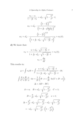
d) We know that:
vY =
u + a
Y ·
1 − u2
c2 · t
1 + u
c2 · a
Y ·
1 − u2
c2 · t
= vY(t);
vY =
dy
dt
.
This results in:
y =
vYdt =
u + a
Y ·
1 − u2
c2 · t
1 + u
c2 · a
Y ·
1 − u2
c2 · t
· dt;
A + B · x
C + D · x
· dx =
1
D
B · x +
Δ
D
· ln |C + D · x|
;
Δ = AD − BC;
A = u; B = a
Y · 1 −
u2
c2
; C = 1;
D =
u
c2
· a
Y · 1 −
u2
c2
; x = t;
Δ =
u2
c2
· a
Y · 1 −
u2
c2
− a
Y · 1 −
u2
c2
= −a
Y · 1 −
u2
c2
·
1 −
u2
c2
;
19.
8 Astronomy andAstrophysics Olympiad - Volume 3
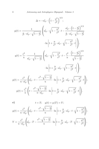
Δ = −a
Y ·
1 −
u2
c2
3/2
;
y(t) =
1
u
c2 · a
Y ·
1 − u2
c2
⎛
⎜
⎝a
Y · 1 −
u2
c2
· t −
a
Y ·
1 − u2
c2
3/2
u
c2 · a
Y ·
1 − u2
c2
· ln
1 +
u
c2
· a
Y · 1 −
u2
c2
· t
⎞
⎟
⎠;
y(t) =
c2
u
·
1
a
Y ·
1 − u2
c2
⎛
⎜
⎝a
Y · 1 −
u2
c2
· t −
c2
u
·
1 − u2
c2
3/2
1 − u2
c2
· ln
1 +
u
c2
· a
Y · 1 −
u2
c2
· t
⎞
⎟
⎠;
y(t) =
c2
u · a
Y
⎛
⎝a
Y · t −
c2 ·
1 − u2
c2
u
· ln
1 +
u
c2
· a
Y · 1 −
u2
c2
· t
⎞
⎠;
y(t) =
c2
u
⎛
⎝t −
c2 ·
1 − u2
c2
u · a
Y
· ln
1 +
u
c2
· a
Y · 1 −
u2
c2
· t
⎞
⎠.
e) t = T; y(t) = y (T) = Y ;
y(t) =
c2
u · a
Y
⎛
⎝a
Y · t −
c2 ·
1 − u2
c2
u
· ln
1 +
u
c2
· a
Y · t · 1 −
u2
c2
⎞
⎠;
Y =
c2
u · a
Y
⎛
⎝a
Y · T −
c2 ·
1 − u2
c2
u
· ln
1 +
u
c2
· a
Y · T · 1 −
u2
c2
⎞
⎠.
20.
A Spaceship toAlpha Centauri 9
f)
t = T; vY(t) = vY(T) = vY,max;
vY =
u + a
Y ·
1 − u2
c2 · t
1 + u
c2 · a
Y ·
1 − u2
c2 · t
= vY(t);
vY,max =
u + a
Y · T ·
1 − u2
c2
1 + u
c2 · a
Y · T ·
1 − u2
c2
.
g)
Y
=
a
Y T2
2
; Y =
Y + uT
1 +
uv
Y,max
c2
; v
Y,max = a
Y T
;
Y =
Y + uT
1 +
ua
Y T
c2
; Y =
a
Y T2
2 + uT
1 +
ua
Y T
c2
;
a
Y T2
2
+ uT
= Y + Y
ua
Y T
c2
;
a
Y T2
− 2u
Y a
Y
c2
− 1
T
− 2Y = 0;
T
=
u
Y a
Y
c2 − 1
+ u2
Y a
Y
c2 − 1
2
+ 2Y a
Y
a
Y
; Y
=
a
Y T2
2
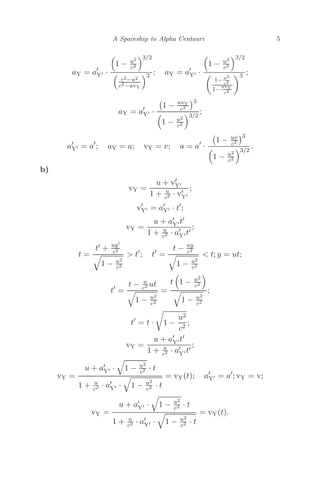
.
h) If u c, then:
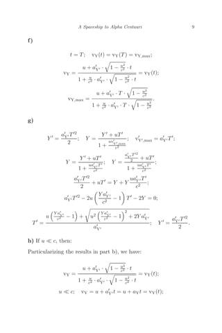
Particularizing the results in part b), we have:
vY =
u + a
Y ·
1 − u2
c2 · t
1 + u
c2 · a
Y ·
1 − u2
c2 · t
= vY(t);
u c; vY = u + a
Y t = u + aYt = vY(t);
21.
10 Astronomy andAstrophysics Olympiad - Volume 3
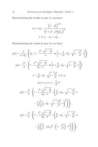
Particularizing the results in part c), we have:
aY = a
Y ·
1 − u2
c2
3/2
1 + u
c2 · vY−u
1− u
c2 ·vY
3 ;
u c; aY = a
Y .
Particularizing the results in part d), we have:
y(t) =
c2
u · a
Y
⎛
⎝a
Y · t −
c2 ·
1 − u2
c2
u
· ln
1 +
u
c2
· a
Y · 1 −
u2
c2
· t
⎞
⎠;
y(t) =
c2
u
·
⎛
⎝t −
c2 ·
1 − u2
c2
a
Y · u
· ln
1 +
u
c2
· a
Y · 1 −
u2
c2
· t
⎞
⎠;
x =
u
c2
· a
Y · 1 −
u2
c2
· t 1;
ln |1 + x| ≈ x −
1
2
x2
;
y(t) =
c2
u
·
⎛
⎝t −
c2 ·
1 − u2
c2
a
Y · u
·
u
c2
· a
Y · 1 −
u2
c2
· t
−
1
2
u
c2
· a
Y · 1 −
u2
c2
· t
2
⎞
⎠
⎞
⎠;
y(t) =
c2
u
·
⎛
⎝t −
c2 ·
1 − u2
c2
a
Y · u
·
u
c2
· a
Y · 1 −
u2
c2
· t
−
1
2
u2
c4
·
a
Y
2
·
1 −
u2
c2
· t2
⎞
⎠
⎞
⎠;
22.
A Spaceship toAlpha Centauri 11
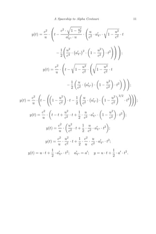
y(t) =
c2
u
·
⎛
⎝t −
c2 ·
1 − u2
c2
a
Y · u
·
u
c2
· a
Y · 1 −
u2
c2
· t
−
1
2
u2
c4
·
a
Y
2
·
1 −
u2
c2
· t2
⎞
⎠
⎞
⎠;
y(t) =
c2
u
·
t − 1 −
u2
c2
·
1 −
u2
c2
· t
−
1
2
u
c2
·
a
Y ·
1 −
u2
c2
· t2
;
y(t) =
c2
u
·
t −
1 −
u2
c2
· t −
1
2
u
c2
·
a
Y ·
1 −
u2
c2
3/2
· t2
;
y(t) =
c2
u
·
t − t +
u2
c2
· t +
1
2
·
u
c2
· a
Y ·
1 −
u2
c2
· t2
;
y(t) =
c2
u
·
u2
c2
· t +
1
2
·
u
c2
· a
Y · t2
;
y(t) =
c2
u
·
u2
c2
· t +
1
2
·
c2
u
·
u
c2
· a
Y · t2
;
y(t) = u · t +
1
2
· a
Y · t2
; a
Y = a
; y = u · t +
1
2
· a
· t2
.
23.
This page intentionallyleft blank
This page intentionally left blank
24.
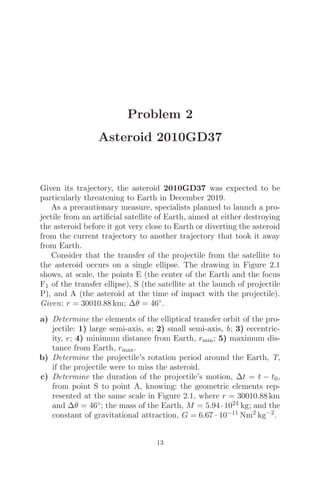
Problem 2
Asteroid 2010GD37
Givenits trajectory, the asteroid 2010GD37 was expected to be
particularly threatening to Earth in December 2019.
As a precautionary measure, specialists planned to launch a pro-
jectile from an artificial satellite of Earth, aimed at either destroying
the asteroid before it got very close to Earth or diverting the asteroid
from the current trajectory to another trajectory that took it away
from Earth.
Consider that the transfer of the projectile from the satellite to
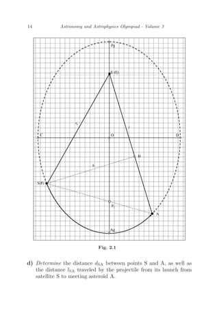
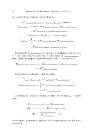
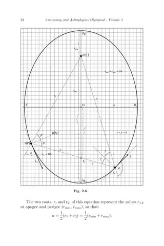
the asteroid occurs on a single ellipse. The drawing in Figure 2.1
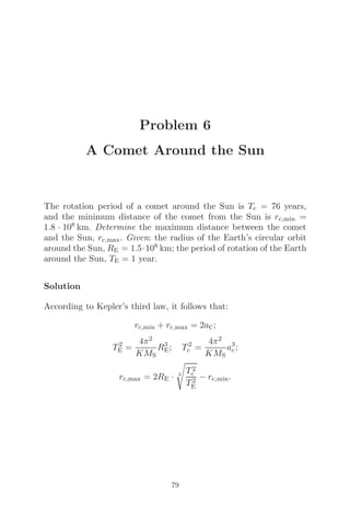
shows, at scale, the points E (the center of the Earth and the focus
F1 of the transfer ellipse), S (the satellite at the launch of projectile
P), and A (the asteroid at the time of impact with the projectile).
Given: r = 30010.88 km; Δθ = 46◦.
a) Determine the elements of the elliptical transfer orbit of the pro-
jectile: 1) large semi-axis, a; 2) small semi-axis, b; 3) eccentric-
ity, e; 4) minimum distance from Earth, rmin; 5) maximum dis-
tance from Earth, rmax.
b) Determine the projectile’s rotation period around the Earth, T,
if the projectile were to miss the asteroid.
c) Determine the duration of the projectile’s motion, Δt = t − t0,
from point S to point A, knowing: the geometric elements rep-
resented at the same scale in Figure 2.1, where r = 30010.88 km
and Δθ = 46◦; the mass of the Earth, M = 5.94·1024 kg; and the
constant of gravitational attraction, G = 6.67 · 10−11 Nm2
kg−2
.
13
25.
14 Astronomy andAstrophysics Olympiad - Volume 3
1
E (F)
S(P)
A
0
r
r
2
F
O
Pg
Ag
C D
H
h
Fig. 2.1
d) Determine the distance dSA between points S and A, as well as
the distance lSA traveled by the projectile from its launch from
satellite S to meeting asteroid A.
26.
Asteroid 2010GD37 15
e)Determine the elements of the velocity vector (orientation and
modulus) of the projectile, P, in relation to the Earth, at the
time of its launch from the circum-terrestrial satellite S, so that
the transfer of the projectile from point S to point A occurs on a
single ellipse,
vellipse =
v0.
f) Determine the projectile’s velocity,
v, orientation, and modulus
on impact with the asteroid, at point A.
g) Evaluate the possibility of observing the projectile with the naked
eye from the surface of the Earth when the projectile is at the
maximum distance from the Earth. We know: the albedo of the
full Moon, αM = 0.12; the radius of the Moon, RM = 1738 km;
the distance from Earth to the Moon, rEM = 384 400 km; and the
apparent magnitude of the full Moon, mM = −12.7m. It is known
that the projectile is a metal sphere with a perfectly reflecting
surface (αProjectile = 1) and with radius RProjectile = 400 mm.
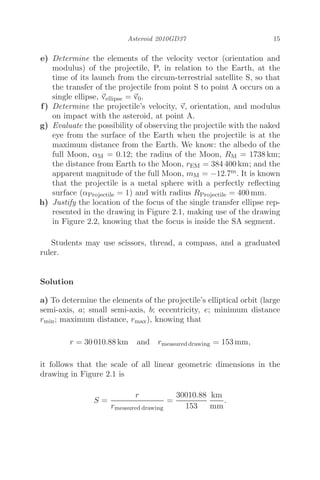
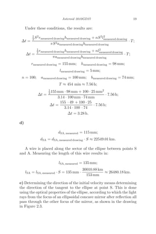
h) Justify the location of the focus of the single transfer ellipse rep-
resented in the drawing in Figure 2.1, making use of the drawing
in Figure 2.2, knowing that the focus is inside the SA segment.
Students may use scissors, thread, a compass, and a graduated
ruler.
Solution
a) To determine the elements of the projectile’s elliptical orbit (large
semi-axis, a; small semi-axis, b; eccentricity, e; minimum distance
rmin; maximum distance, rmax), knowing that
r = 30 010.88 km and rmeasured drawing = 153 mm,
it follows that the scale of all linear geometric dimensions in the
drawing in Figure 2.1 is
S =
r
rmeasured drawing
=
30010.88
153
km
mm
.
27.
16 Astronomy andAstrophysics Olympiad - Volume 3
S(P)
A
0
r
r
θ
Δ
d
1
E(F)
Fig. 2.2
28.
Asteroid 2010GD37 17
So,we get:
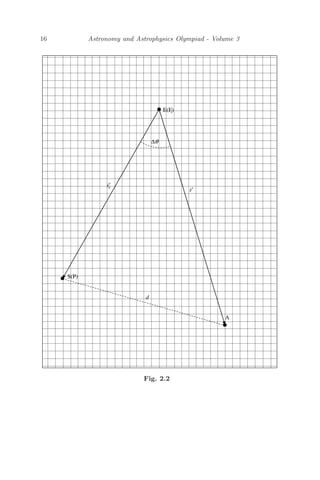
r0, measured = 133 mm; r0 = r0, measured drawing · S = 26087.88 km;
rmeasured = 153 mm;
2ameasured drawing = 200 mm; ameasured drawing = 100 mm;
a = ameasured drawing · S ≈ 19614.95 km;
2bmeasured drawing = 148 mm; bmeasured drawing = 74 mm;
b = bmeasured drawing · S ≈ 14515.06 km;
2cmeasured drawing = 134 mm; cmeasured drawing = 67 mm;
c = cmeasured drawing · S ≈ 13142.01 km;
e =
1 −
b2
a2
=
1 −
b2
measured drawing
a2
measured drawing
≈ 0.67;
rmin, measured drawing = 33 mm;
rmin = rmin, measured drawing · S ≈ 6472.93 km; rmin = a(1 − e);
rmax, measured drawing = 167 mm;
rmax = rmax, measured · S ≈ 32756.97 km; rmax = a(1 + e).
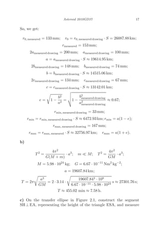
b)
T2
=
4π2
G(M + m)
· a3
; m M; T2
=
4π2
GM
· a3
;
M = 5.98 · 1024
kg; G = 6.67 · 10−11
Nm2
kg−2
;
a = 19607.84 km;
T = 2π
a3
GM
= 2 · 3.14 ·
19607.843 · 109
6.67 · 10−11 · 5.98 · 1024
s ≈ 27301.76 s;
T ≈ 455.02 min ≈ 7.58 h.
c) On the transfer ellipse in Figure 2.1, construct the segment
SH ⊥ EA, representing the height of the triangle ESA, and measure
29.
18 Astronomy andAstrophysics Olympiad - Volume 3
the length of this segment on the drawing:
(SH)measured drawing = hmeasured drawing = 98 mm;
Σellipse transfer = πab = πSameasured drawing · Sbmeasured drawing
= πS2
ameasured drawingbmeasured drawing;
Σsector ellipse = ΣΔ(ESA) + Σsegment ellipse;
ΣΔ(ESA) =
1
2
rh =
1
2
Srmeasured drawingShmeasured drawing
=
1
2
S2
rmeasured drawinghmeasured drawing.
To calculate Σsegment ellipse by counting, we estimate that there are
n = 100 small squares, each with a side length of lmeasured drawing =
5 mm. Thus, corresponding to the same scale, S, the result is:
Σsegment ellipse transfer = n · Slmeasured drawing · Slmeasured drawing
= nS2
l2
measured drawing.
Under these conditions, it follows that:
Σsector ellipse transfer = ΣΔ(ESA) + Σsegment ellipse;
Σsector ellipse transfer =
1
2
S2
rmeasured drawinghmeasured drawing
+ nS2
l2
measured drawing.
According to Kepler’s second law (the law of areas), it follows
that:
T................................. Σtransfer ellipse;
Δt ......................... Σsector ellipse transfer;
Δt =
Σsector ellipse transfer
Σtransfer ellipse
· T,
representing the duration of projectile P’s displacement until it meets
asteroid A.
30.
Asteroid 2010GD37 19
Underthese conditions, the results are:
Δt =
1
2S2rmeasured drawinghmeasured drawing + nS2l2
measured drawing
πS2ameasured drawingbmeasured drawing
· T;
Δt =
1
2 rmeasured drawinghmeasured drawing + nl2
measured drawing
πameasured drawingbmeasured drawing
· T;
rmeasured drawing = 155 mm; hmeasured drawing = 98 mm;
lmeasured drawing = 5 mm;
n = 100; ameasured drawing = 100 mm; bmeasured drawing = 74 mm;
T ≈ 454 min ≈ 7.56 h;
Δt =
1
2 155 mm · 98 mm + 100 · 25 mm2
3.14 · 100 mm · 74 mm
· 7.56 h;
Δt =
155 · 49 + 100 · 25
3.14 · 100 · 74
· 7.56 h;
Δt = 3.28 h.
d)
dSA, measured = 115 mm;
dSA = dSA, measured drawing · S ≈ 22549.01 km.
A wire is placed along the sector of the ellipse between points S
and A. Measuring the length of this wire results in:
lSA, measured = 135 mm;
lSA = lSA, measured · S = 135 mm ·
30010.88 km
153 mm
≈ 26480.18 km.
e) Determining the direction of the initial velocity means determining
the direction of the tangent to the ellipse at point S. This is done
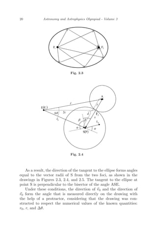
using the optical properties of the ellipse, according to which the light
rays from the focus of an ellipsoidal concave mirror after reflection all
pass through the other focus of the mirror, as shown in the drawing
in Figure 2.3.
31.
20 Astronomy andAstrophysics Olympiad - Volume 3
1
F 2
F
Fig. 2.3
Fig. 2.4
As a result, the direction of the tangent to the ellipse forms angles
equal to the vector radii of S from the two foci, as shown in the
drawings in Figures 2.3, 2.4, and 2.5. The tangent to the ellipse at
point S is perpendicular to the bisector of the angle ASE.
Under these conditions, the direction of
v0 and the direction of
r0 form the angle that is measured directly on the drawing with
the help of a protractor, considering that the drawing was con-
structed to respect the numerical values of the known quantities:
r0, r, and Δθ.
32.
Asteroid 2010GD37 21
Fig.2.5
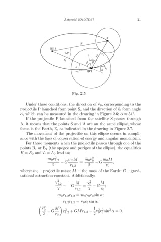
Under these conditions, the direction of
v0, corresponding to the
projectile P launched from point S, and the direction of
r0 form angle
α, which can be measured in the drawing in Figure 2.6: α ≈ 54◦.
If the projectile P launched from the satellite S passes through
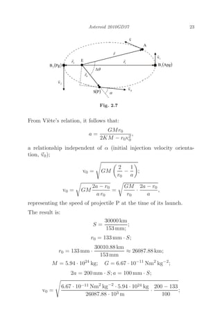
A, it means that the points S and A are on the same ellipse, whose
focus is the Earth, E, as indicated in the drawing in Figure 2.7.
The movement of the projectile on this ellipse occurs in compli-
ance with the laws of conservation of energy and angular momentum.
For those moments when the projectile passes through one of the
points B1 or B2 (the apogee and perigee of the ellipse), the equalities
E = E0 and L = L0 lead to:
m0v2
1,2
2
− G
m0M
r1,2
=
m0v2
0
2
− G
m0M
r0
,
where: m0 – projectile mass; M – the mass of the Earth; G – gravi-
tational attraction constant. Additionally:
v2
1,2
2
− G
M
r1,2
=
v2
0
2
− G
M
r0
;
m0v1,2r1,2 = m0v0r0 sin α;
v1,2r1,2 = v0r0 sin α;
v2
0
2
− G
M
r0
r2
1,2 + GMr1,2 −
1
2
v2
0r2
0 sin2
α = 0.
33.
22 Astronomy andAstrophysics Olympiad - Volume 3
Fig. 2.6
The two roots, r1 and r2, of this equation represent the values r1,2
at apogee and perigee (rmin, rmax), so that:
a =
1
2
(r1 + r2) =
1
2
(rmin + rmax).
34.
Asteroid 2010GD37 23
Fig.2.7
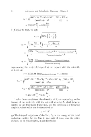
From Viète’s relation, it follows that:
a =
GMr0
2KM − r0v2
0
,
a relationship independent of α (initial injection velocity orienta-
tion,
v0);
v0 =
GM
2
r0
−
1
a
;
v0 =
GM
2a − r0
a r0
=
GM
r0
·
2a − r0
a
,
representing the speed of projectile P at the time of its launch.
The result is:
S =
30000 km
153 mm;
;
r0 = 133 mm · S;
r0 = 133 mm ·
30010.88 km
153 mm
≈ 26087.88 km;
M = 5.94 · 1024
kg; G = 6.67 · 10−11
Nm2
kg−2
;
2a = 200 mm · S; a = 100 mm · S;
v0 =
6.67 · 10−11 Nm2
kg−2
· 5.94 · 1024 kg
26087.88 · 103 m
·
200 − 133
100
;
35.
24 Astronomy andAstrophysics Olympiad - Volume 3
v0 =
6.67 · 10−11 · 5.94 · 1024
26087.88 · 103
·
200 − 133
100
m
s
≈ 3189.87
m
s
= 3.18
km
s
.
f) Similar to that, we get:
vA =
GM
2
r
−
1
a
;
vA =
GM
2
r
−
1
a
=
GM
2a − r
ar
=
GM
r
·
2ameasured drawing · S − rmeasured drawing · S
ameasured drawing · S
;
vA =
GM
r
·
2ameasured drawing − rmeasured drawing
ameasured drawing
,
representing the projectile’s speed at the impact with the asteroid,
at point A;
r = 30010.88 km; rmeasured drawing = 153 mm;
vA =
6.67 · 10−11 Nm2
kg−2
· 5.94 · 1024 kg
30010.88 · 103 m
·
200 − 153
100
;
vA =
6.67 · 10−11 · 5.94 · 1024
30010.88 · 103
·
200 − 153
100
m
s
≈ 2974.09
m
s
≈ 2.97
km
s
.
Under these conditions, the direction of
v, corresponding to the
impact of the projectile with the asteroid at point A, which is high-
lighted in the drawing in Figure 2.6, and the direction of
r form the
angle ϕ, whose value can be measured as:
ϕ ≈ 118◦
.
g) The integral brightness of the Sun, LS, is the energy of the total
radiation emitted by the Sun in one unit of time, over its entire
surface, on all wavelengths, in all directions:
36.
Asteroid 2010GD37 25
LS=
Eemitted, Sun
t
= 3.86 · 1026
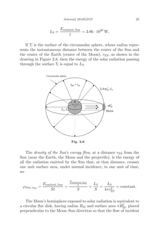
W,
If Σ is the surface of the circumsolar sphere, whose radius repre-
sents the instantaneous distance between the center of the Sun and
the center of the Earth (center of the Moon), rES, as shown in the
drawing in Figure 2.8, then the energy of the solar radiation passing
through the surface Σ is equal to LS.
Fig. 2.8
The density of the Sun’s energy flow, at a distance rES from the
Sun (near the Earth, the Moon and the projectile), is the energy of
all the radiation emitted by the Sun that, at that distance, crosses
one unit surface area, under normal incidence, in one unit of time,
so:
ϕSun, rES
=
Eemitted, Sun
St
=
Eemitted, Sun
t
S
=
LS
S
=
LS
4πr2
ES
= constant.
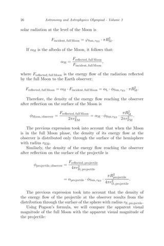
The Moon’s hemisphere exposed to solar radiation is equivalent to
a circular flat disk, having radius RM and surface area πR2
M, placed
perpendicular to the Moon–Sun direction so that the flow of incident
37.
26 Astronomy andAstrophysics Olympiad - Volume 3
solar radiation at the level of the Moon is
Fincident, full Moon = ϕSun, rES
· πR2
M.
If αM is the albedo of the Moon, it follows that:
αM =
Freflected, full Moon
Fincident, full Moon
,
where Freflected, full Moon is the energy flow of the radiation reflected
by the full Moon to the Earth observer;
Freflected, full Moon = αM · Fincident, full Moon = αL · φSun, rES
· πR2
M.
Therefore, the density of the energy flow reaching the observer
after reflection on the surface of the Moon is
φMoon, observer =
Freflected, full Moon
2πr2
EM
= αM · φSun,rES
·
πR2
M
2πr2
PM
.
The previous expression took into account that when the Moon
is in the full Moon phase, the density of its energy flow at the
observer is distributed only through the surface of the hemisphere
with radius rEM.
Similarly, the density of the energy flow reaching the observer
after reflection on the surface of the projectile is
φprojectile, observer =
Freflected, projectile
4πr2
D, projectile
= αprojectile · φSun, rES
·
πR2
projectile
4πr2
D, projectile
.
The previous expression took into account that the density of
the energy flow of the projectile at the observer results from the
distribution through the surface of the sphere with radius rE, projectile.
Using Pogson’s formula, we will compare the apparent visual
magnitude of the full Moon with the apparent visual magnitude of
the projectile:
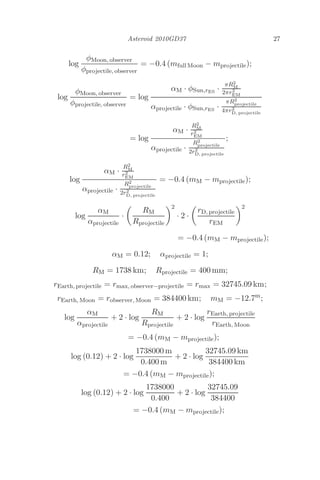
28 Astronomy andAstrophysics Olympiad - Volume 3
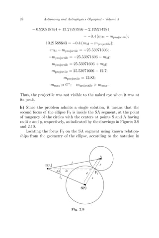
− 0.920818754 + 13.27597956 − 2.139274381
= −0.4 (mM − mprojectile);
10.21588643 = −0.4 (mM − mprojectile);
mM − mprojectile = −25.53971606;
−mprojectile = −25.53971606 − mM;
mprojectile = 25.53971606 + mM;
mprojectile = 25.53971606 − 12.7;
mprojectile = 12.83;
mmax ≈ 6m
; mprojectile mmax.
Thus, the projectile was not visible to the naked eye when it was at
its peak.
h) Since the problem admits a single solution, it means that the
second focus of the ellipse F2 is inside the SA segment, at the point
of tangency of the circles with the centers at points S and A having
radii x and y, respectively, as indicated by the drawings in Figures 2.9
and 2.10.
Locating the focus F2 on the SA segment using known relation-
ships from the geometry of the ellipse, according to the notation in
Fig. 2.9
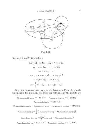
40.
Asteroid 2010GD37 29
Fig.2.10
Figures 2.9 and 2.10, results in:
ES + SF2 = 2a; EA + AF2 = 2a;
r0 + x = 2a; r + y = 2a;
r0 + x = r + y;
x − y = r − r0 = d0; x + y = d;
x − y = d0; x + y = d;
x =
1
2
(d + d0); y =
1
2
(d − d0).
From the measurements made on the drawing in Figure 2.1, in the
statement of the problem, and from our calculations, the results are:
r0, measured drawing = 133 mm; rmeasured drawing = 153 mm;
dmeasured drawing = 115 mm;
d0, calculated drawing = rmeasured drawing − r0, measured drawing = 20 mm;
xcalculated drawing =
1
2
(dmeasured drawing + d0, calculated drawing);
ycalculated drawing =
1
2
(dmeasured − d0, calculated drawing);
xcalculated drawing = 67.5 mm; ycalculated drawing = 47.5 mm.
41.
30 Astronomy andAstrophysics Olympiad - Volume 3
Thus:
xmeasured = 67.5 mm; ymeasured = 47.5 mm,
which allows the location of the focus F2 in the drawing in Figure 2.2,
as shown in the drawing in Figure 2.10.
42.
Problem 3
A Galaxyof Stars Identical
to Our Sun!
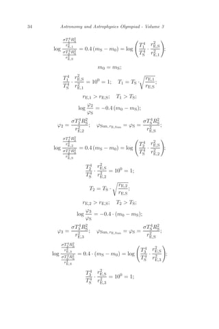
A science fiction hypothesis proposes the possibility of, beyond the
limits of our galaxy, a galaxy whose stars have radii identical and
equal to the radius of our Sun.
In addition, observed from Earth, all the stars of this galaxy would
have identical apparent magnitudes, equal to the apparent magnitude
of our Sun, regardless of the distances at which they would be from
Earth.
Establish the relationships between the effective temperatures of
the surfaces of the stars in this galaxy and the distances at which
they would be from the observer on Earth.
Given: TS – the effective temperature at the surface of the Sun;
rES – the distance between the Earth and the Sun.
Solution
Knowing the relationship between the illumination produced by a
star (the energy flux density of the star, ϕΣ,rEΣ
, at the distance from
the star rEΣ, i.e., at the observer on Earth), the brightness of the
star, LΣ, and the distance between the Earth and the star, rEΣ, we
obtain:
ϕΣ,rEΣ
=
LΣ
4πr2
EΣ
,
31
43.
32 Astronomy andAstrophysics Olympiad - Volume 3
where the brightness of the star, depending on its temperature and
its radius, is given by the expression
LΣ = σT4
Σ4πR2
Σ,
where σ is the constant from the Stefan–Boltzmann law;
ϕΣ,rEΣ
=
σT4
ΣR2
Σ
r2
EΣ
;
log
ϕΣ,rEΣ
ϕSun, rE,Sun
= −0.4 (mΣ − mSun);
mΣ = m0;
log
ϕΣ,rEΣ
ϕSun,rE Sun
= −0.4 (m0 − mSun),
representing Pogson’s formula for the star Σ–Sun ensemble.
Writing the same formula for the ensemble formed by another star
Σ and the Sun:
log
ϕΣ,rEΣ
ϕSun, rE,Sun
= −0.4 (mΣ − mSun);
mΣ = m0;
log
ϕΣ,rEΣ
ϕSun, rE,Sun
= −0.4 (m0 − mSun);
log
ϕΣ,rEΣ
ϕSun, rE,Sun
= log
ϕΣ,rE,Σ
ϕSun, rE,Sun
;
ϕΣ,rEΣ
ϕSun, rE,Sun
=
ϕΣ,rEΣ
ϕSun, rE,Sun
;
ϕΣ,rEΣ
= ϕΣrEΣ .
This proves that, under the conditions of the statement of the
problem:
• The energy flow densities of all stars, at the level of the observer
44.
A Galaxy ofStars Identical to Our Sun! 33
on Earth, are identical, which is why the apparent magnitudes of
all stars in the “Galaxy of Exoplanets” are identical, m0:
ϕ1,rE,1
= ϕ2,rE,2
= ϕ3,rE,3
= · · · · · · = ϕN,rE,N
;
σT4
1 R2
1
r2
E,1
=
σT4
2 R2
2
r2
E,2
=
σT4
3 R2
3
r2
E,3
= · · · · · · · · · =
σT4
N R2
N
r2
E,N
.
• The luminosities (absolute luminosities) of the stars must be
higher, at greater distances from the Earth, so the apparent mag-
nitudes of all the stars in the “Galaxy of Exoplanets” can remain
unchanged, m0:
LΣ = σT4
Σ4πR2
Σ;
L1 = σT4
1 4πR2
1; L2 = σT4
2 4πR2
2; L3 = σT4
3 4πR2
3; . . . . . . . . . ;
LN = σT4
N 4πR2
N ;
L1 L2 L3 · · · · · · · · · LN ;
σT4
1 4πR2
1 σT4
2 4πR2
2 σT4
3 4πR2
3 · · · · · · · · · σT4
N 4πR2
N ;
T4
1 R2
1 T4
2 R2
2 T4
3 R2
3 · · · · · · · · · T4
N R2
N .
R1 = R2 = R3 = · · · · · · · · · = RN = RS;
T4
1 T4
2 T4
3 · · · · · · · · · T4
N ;
T1 T2 T3 · · · · · · · · · TN .
That is, the luminosities of the stars increase when the distances
between the Earth and the stars increase because the temperatures
of the stars become higher, which can cause the apparent magnitudes
of the stars to be constant.
Under these conditions, writing Pogson’s formula for each ensem-
ble (star–Sun) results in:
log
ϕ1
ϕS
= −0.4 (m0 − mS);
ϕ1 =
σT4
1 R2
S
r2
E,1
; ϕSun, rE,Sun
= ϕS =
σT4
S R2
S
r2
E,S
;
A Galaxy ofStars Identical to Our Sun! 35
T3 = TS ·
rE,3
rE,S
;
rE,3 rE,S; T3 TS;
...............................................................
log
ϕN
ϕS
= −0.4 · (m0 − mS); ϕN =
σT4
N R2
S
r2
E,N
;
ϕSun,rE,Sun
= ϕS =
σT4
S R2
S
r2
E,S
;
log
σT4
N R2
S
r2
E,N
σT2
S R2
S
r2
E,S
= 0.4 · (mS − m0) = log
T4
N
T4
S
·
r2
E,S
r2
E,N
;
T4
N
T4
S
·
r2
E,S
r2
E,N
= 100
= 1;
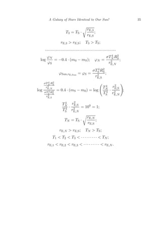
TN = TS ·
rE,N
rE,S
;
rE,N rE,S; TN TS;
T1 T2 T3 · · · · · · · · · TN ;
rE,1 rE,2 rE,3 · · · · · · · · · rE,N .
47.
This page intentionallyleft blank
This page intentionally left blank
48.
Problem 4
Two AstronomicalObservatories
on an Island
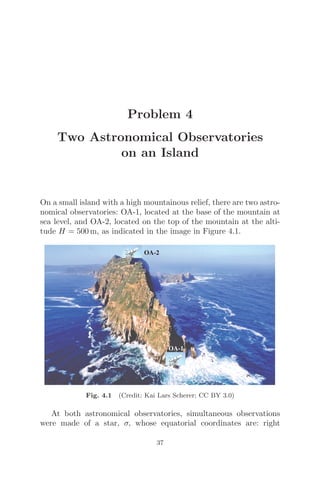
On a small island with a high mountainous relief, there are two astro-
nomical observatories: OA-1, located at the base of the mountain at
sea level, and OA-2, located on the top of the mountain at the alti-
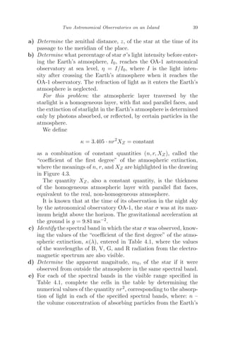
tude H = 500 m, as indicated in the image in Figure 4.1.
OA-1
OA-2
Fig. 4.1 (Credit: Kai Lars Scherer; CC BY 3.0)
At both astronomical observatories, simultaneous observations
were made of a star, σ, whose equatorial coordinates are: right
37
49.
38 Astronomy andAstrophysics Olympiad - Volume 3
ascension, α = 01h10m36s; declination, δ = 12◦3000. The geo-
graphical coordinates of the island are: north latitude, ϕ = 43◦; west
longitude, λ = 61◦.
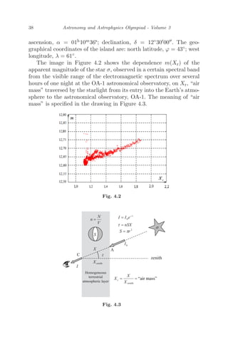
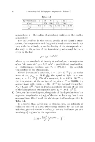
The image in Figure 4.2 shows the dependence m(Xr) of the
apparent magnitude of the star σ, observed in a certain spectral band
from the visible range of the electromagnetic spectrum over several
hours of one night at the OA-1 astronomical observatory, on Xr, “air
mass” traversed by the starlight from its entry into the Earth’s atmo-
sphere to the astronomical observatory, OA-1. The meaning of “air
mass” is specified in the drawing in Figure 4.3.
Fig. 4.2
“air mass”
Fig. 4.3
50.
Two Astronomical Observatorieson an Island 39
a) Determine the zenithal distance, z, of the star at the time of its
passage to the meridian of the place.
b) Determine what percentage of star σ’s light intensity before enter-
ing the Earth’s atmosphere, I0, reaches the OA-1 astronomical
observatory at sea level, η = I/I0, where I is the light inten-
sity after crossing the Earth’s atmosphere when it reaches the
OA-1 observatory. The refraction of light as it enters the Earth’s
atmosphere is neglected.
For this problem: the atmospheric layer traversed by the
starlight is a homogeneous layer, with flat and parallel faces, and
the extinction of starlight in the Earth’s atmosphere is determined
only by photons absorbed, or reflected, by certain particles in the
atmosphere.
We define
κ = 3.405 · nr2
XZ = constant
as a combination of constant quantities (n, r, XZ ), called the
“coefficient of the first degree” of the atmospheric extinction,
where the meanings of n, r, and XZ are highlighted in the drawing
in Figure 4.3.
The quantity XZ, also a constant quantity, is the thickness
of the homogeneous atmospheric layer with parallel flat faces,
equivalent to the real, non-homogeneous atmosphere.
It is known that at the time of its observation in the night sky
by the astronomical observatory OA-1, the star σ was at its max-
imum height above the horizon. The gravitational acceleration at
the ground is g = 9.81 ms−2.
c) Identify the spectral band in which the star σ was observed, know-
ing the values of the “coefficient of the first degree” of the atmo-
spheric extinction, κ(λ), entered in Table 4.1, where the values
of the wavelengths of B, V, G, and R radiation from the electro-
magnetic spectrum are also visible.
d) Determine the apparent magnitude, m0, of the star if it were
observed from outside the atmosphere in the same spectral band.
e) For each of the spectral bands in the visible range specified in
Table 4.1, complete the cells in the table by determining the
numerical values of the quantity nr2, corresponding to the absorp-
tion of light in each of the specified spectral bands, where: n –
the volume concentration of absorbing particles from the Earth’s
51.
40 Astronomy andAstrophysics Olympiad - Volume 3
Table 4.1
Spectral band U B V G R I
λ(nm) 470 550 600 780
κ(λ) 0.6 0.4 0.2 0.166 0.1 0.08
nr2
atmosphere; r – the radius of absorbing particles in the Earth’s
atmosphere.
For this problem: in the vertical profile of the Earth’s atmo-
sphere, the temperature and the gravitational acceleration do not
vary with the altitude, h, so the density of the atmospheric air,
due only to the action of the terrestrial gravitational forces, is
given by the law
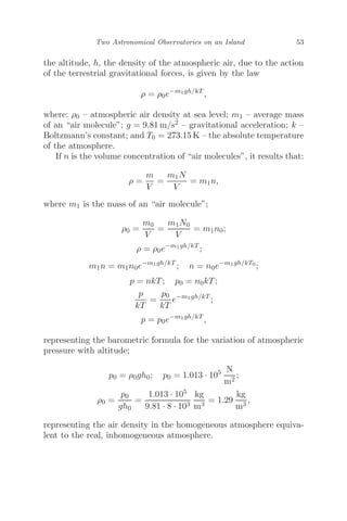
ρ = ρ0e−m1gh/kT
,
where: ρ0 – atmospheric air density at sea level; m1 – average mass
of an “air molecule”; g = 9.81 m/s2 – gravitational acceleration;
k – Boltzmann’s constant; and T0 = 273.15 K – the absolute
temperature of the atmosphere.
Given: Boltzmann’s constant, k = 1.38 · 10−23 J
K ; the molar
mass of air, μair = 28.96 g
mol; the speed of light in a vac-
uum, c = 3 · 108 m
s ; Planck’s constant, h = 6.625 · 10−34 Js;
the temperature at the surface of the star σ, T = 6000 K; the
atomic mass unit, 1 amu = 1.66 · 10−27 kg; Avogadro’s number,
NA = 6.023·1023 1/mol; and the atmospheric pressure at the base
of the homogeneous atmospheric layer, p0 = 1.013 · 105 N
m2 .
f) Draw, on the same diagram, the graphs of the dependences of the
apparent magnitudes, m(Xr), of the star σ, knowing that it was
observed from OA-1 in all the visible spectral bands specified in
Table 4.1.
It is known that, according to Planck’s law, the intensity of
radiation emitted by a star (the energy emitted by the star per
unit time, per unit area of a surface, at normal incidence, per unit
wavelength) is given by the expression
I0(λ) =
2hc2
λ5
ehc/kλT
− 1
−1
.
52.
Two Astronomical Observatorieson an Island 41
g) Determine the zenithal distance of the star σ for which two of the
four visual apparent magnitudes, corresponding to the four visual
spectral bands (B, V, G, R), are identical for the OA-1 observer.
h) Determine what percentage of star σ’s light intensity before enter-
ing the Earth’s atmosphere, I0, reaches the OA-2 astronomical
observatory from altitude H, η = I/I0.
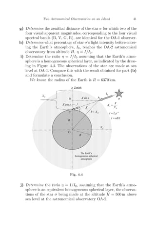
i) Determine the ratio η = I/I0 assuming that the Earth’s atmo-
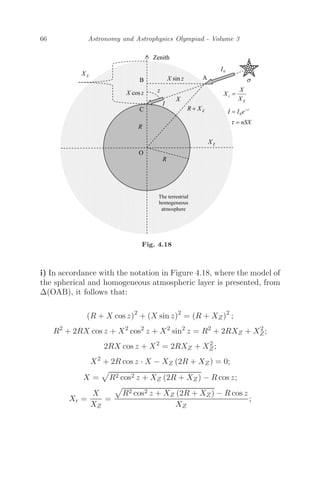
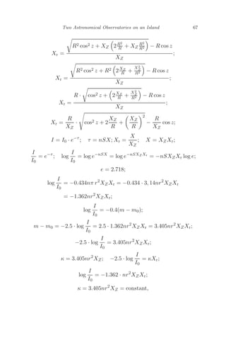
sphere is a homogeneous spherical layer, as indicated by the draw-
ing in Figure 4.4. The observations of the star are made at sea
level at OA-1. Compare this with the result obtained for part (b)
and formulate a conclusion.
We know: the radius of the Earth is R = 6370 km.
Fig. 4.4
j) Determine the ratio η = I/I0, assuming that the Earth’s atmo-
sphere is an equivalent homogeneous spherical layer, the observa-
tions of the star σ being made at the altitude H = 500 m above
sea level at the astronomical observatory OA-2.
53.
42 Astronomy andAstrophysics Olympiad - Volume 3
Solution
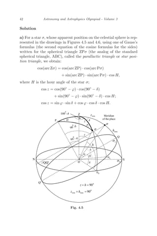
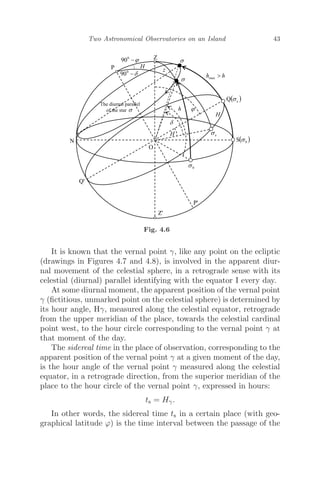
a) For a star σ, whose apparent position on the celestial sphere is rep-
resented in the drawings in Figures 4.5 and 4.6, using one of Gauss’s
formulas (the second equation of the cosine formulas for the sides)
written for the spherical triangle ZPσ (the analog of the standard
spherical triangle, ABC), called the parallactic triangle or star posi-
tion triangle, we obtain:
cos(arc Zσ) = cos(arc ZP) · cos(arc Pσ)
+ sin(arc ZP) · sin(arc Pσ) · cos H,
where H is the hour angle of the star σ;
cos z = cos(90◦
− ϕ) · cos(90◦
− δ)
+ sin(90◦
− ϕ) · sin(90◦
− δ) · cos H;
cos z = sin ϕ · sin δ + cos ϕ · cos δ · cos H.
Fig. 4.5
54.
Two Astronomical Observatorieson an Island 43
Fig. 4.6
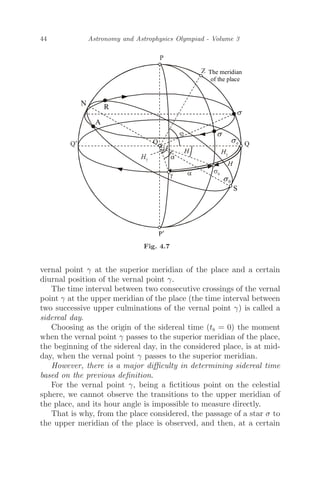
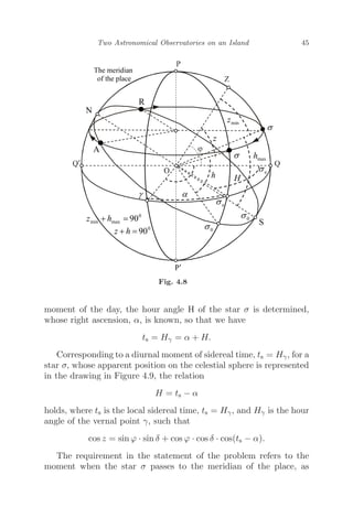
It is known that the vernal point γ, like any point on the ecliptic
(drawings in Figures 4.7 and 4.8), is involved in the apparent diur-
nal movement of the celestial sphere, in a retrograde sense with its
celestial (diurnal) parallel identifying with the equator I every day.
At some diurnal moment, the apparent position of the vernal point
γ (fictitious, unmarked point on the celestial sphere) is determined by
its hour angle, Hγ, measured along the celestial equator, retrograde
from the upper meridian of the place, towards the celestial cardinal
point west, to the hour circle corresponding to the vernal point γ at
that moment of the day.
The sidereal time in the place of observation, corresponding to the
apparent position of the vernal point γ at a given moment of the day,
is the hour angle of the vernal point γ measured along the celestial
equator, in a retrograde direction, from the superior meridian of the
place to the hour circle of the vernal point γ, expressed in hours:
ts = Hγ.
In other words, the sidereal time ts in a certain place (with geo-
graphical latitude ϕ) is the time interval between the passage of the
55.
44 Astronomy andAstrophysics Olympiad - Volume 3
Fig. 4.7
vernal point γ at the superior meridian of the place and a certain
diurnal position of the vernal point γ.
The time interval between two consecutive crossings of the vernal
point γ at the upper meridian of the place (the time interval between
two successive upper culminations of the vernal point γ) is called a
sidereal day.
Choosing as the origin of the sidereal time (ts = 0) the moment
when the vernal point γ passes to the superior meridian of the place,
the beginning of the sidereal day, in the considered place, is at mid-
day, when the vernal point γ passes to the superior meridian.
However, there is a major difficulty in determining sidereal time
based on the previous definition.
For the vernal point γ, being a fictitious point on the celestial
sphere, we cannot observe the transitions to the upper meridian of
the place, and its hour angle is impossible to measure directly.
That is why, from the place considered, the passage of a star σ to
the upper meridian of the place is observed, and then, at a certain
56.
Two Astronomical Observatorieson an Island 45
Fig. 4.8
moment of the day, the hour angle H of the star σ is determined,
whose right ascension, α, is known, so that we have
ts = Hγ = α + H.
Corresponding to a diurnal moment of sidereal time, ts = Hγ, for a
star σ, whose apparent position on the celestial sphere is represented
in the drawing in Figure 4.9, the relation
H = ts − α
holds, where ts is the local sidereal time, ts = Hγ, and Hγ is the hour
angle of the vernal point γ, such that
cos z = sin ϕ · sin δ + cos ϕ · cos δ · cos(ts − α).
The requirement in the statement of the problem refers to the
moment when the star σ passes to the meridian of the place, as
57.
46 Astronomy andAstrophysics Olympiad - Volume 3
Fig. 4.9
indicated by the drawing in Figure 4.10, when its height above the
horizon is maximum, hmax. As a result, the local sidereal time of the
occurrence of this event is ts = 0, such that:
H = ts − α = −α;
cos z = sin ϕ · sin δ + cos ϕ · cos δ · cos(−α);
cos z = sin ϕ · sin δ + cos ϕ · cos δ · cos α;
α = 01h
10m
36s
= 17.65◦
; δ = 12◦
30
00
= 12.5◦
; ϕ = 43◦
;
sin ϕ = 0.681; cos ϕ = 0.731;
sin δ = 0.216; cos δ = 0.976;
cos α = 0.952;
cos z = 0.681 · 0.216 + 0.731 · 0.976 · 0.952 = 0.826;
z ≈ 34◦
.
b) An effect that must be corrected for when calibrating the instru-
mental magnitudes of stars is the atmospheric extinction of radiation,
58.
Two Astronomical Observatorieson an Island 47
Fig. 4.10
or the diminution of starlight due to passage through the Earth’s
atmosphere. The longer the path of starlight through the Earth’s
atmosphere, the greater the extinction of the starlight. As a result,
on the same night, from the moment a star rises, being close to the
horizon (zmax = 90◦), until the moment it reaches the zenith (z = 0),
the distance traveled by the light through the Earth’s atmosphere
decreases, so that the star becomes brighter (its instrumental mag-
nitude becomes smaller).
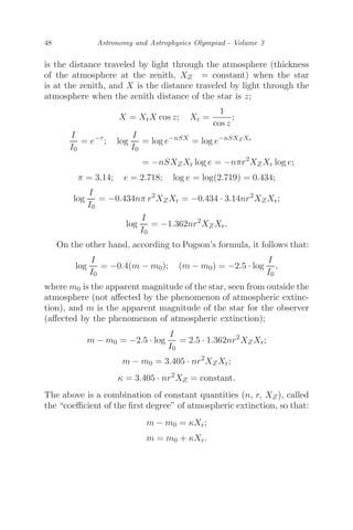
For the study of the extinction of stellar radiation due to its selec-
tive absorption by particles in the Earth’s atmosphere, using the
drawing in Figure 4.3 and knowing the empirical formula of the law
of absorption, we obtain:
I = I0 · e−τ
; τ = nSX; n =
N
V
; S = πr2
; X = XrXZ;
Xzenith = X cos z = XZ,
where r is the radius of absorbing particles in the atmosphere, n
is the concentration of absorbing particles in the atmosphere, XZ
59.
48 Astronomy andAstrophysics Olympiad - Volume 3
is the distance traveled by light through the atmosphere (thickness
of the atmosphere at the zenith, XZ = constant) when the star
is at the zenith, and X is the distance traveled by light through the
atmosphere when the zenith distance of the star is z;
X = XrX cos z; Xr =
1
cos z
;
I
I0
= e−τ
; log
I
I0
= log e−nSX
= log e−nSXZXr
= −nSXZXr log e = −nπr2
XZXr log e;
π = 3.14; e = 2.718; log e = log(2.719) = 0.434;
log
I
I0
= −0.434nπ r2
XZXr = −0.434 · 3.14nr2
XZXr;
log
I
I0
= −1.362nr2
XZXr.
On the other hand, according to Pogson’s formula, it follows that:
log
I
I0
= −0.4(m − m0); (m − m0) = −2.5 · log
I
I0
,
where m0 is the apparent magnitude of the star, seen from outside the
atmosphere (not affected by the phenomenon of atmospheric extinc-
tion), and m is the apparent magnitude of the star for the observer
(affected by the phenomenon of atmospheric extinction);
m − m0 = −2.5 · log
I
I0
= 2.5 · 1.362nr2
XZXr;
m − m0 = 3.405 · nr2
XZXr;
κ = 3.405 · nr2
XZ = constant.
The above is a combination of constant quantities (n, r, XZ), called
the “coefficient of the first degree” of atmospheric extinction, so that:
m − m0 = κXr;
m = m0 + κXr.
60.
Two Astronomical Observatorieson an Island 49
This proves that the magnitude of the star for the observer on the
surface of the Earth, OA-1, after the extinction of the light in the
atmosphere, is a function of the parameter
Xr = “air mass”,
whose physical meaning is that of the “relative” distance traveled by
light from entering the Earth’s atmosphere to the observer:
Xr =
X
Xzenith
,
that is, the ratio of the distance traveled by starlight through the
atmosphere to the observer, when the star is at some position in the
sky, to the distance traveled by starlight through the atmosphere to
the observer when the star is at the observer’s zenith;
Xr ≥ 1;
m(Xr) = m0 + κXr.
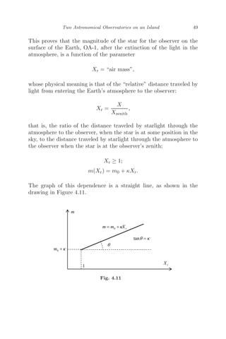
The graph of this dependence is a straight line, as shown in the
drawing in Figure 4.11.
Fig. 4.11
61.
50 Astronomy andAstrophysics Olympiad - Volume 3
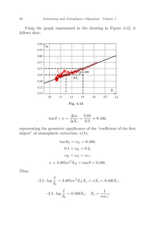
Using the graph represented in the drawing in Figure 4.12, it
follows that:
Fig. 4.12
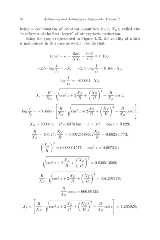
tan θ = κ =
Δm
ΔXr
=
0.05
0.3
≈ 0.166,
representing the geometric significance of the “coefficient of the first
degree” of atmospheric extinction, κ(λ);
tan θG = κG = 0.166;
0.1 κG 0.2;
κR κG κV;
κ = 3.405nr2
XZ = tan θ = 0.166.
Thus:
−2.5 · log
I
I0
= 3.405nr2
XZXr = κXr = 0.166Xr;
−2.5 · log
I
I0
= 0.166Xr; Xr =
1
cos z
;
62.
Two Astronomical Observatorieson an Island 51
−2.5 · log
I
I0
=
0.166
cos z
=
0.166
cos 34◦
=
0.166
0.829
;
log
I
I0
= −
0.166
0.829 · 2.5
= −0.08;
η =
I
I0
= 0.83; I = 0.83 · I0.
c) Locating the value of the coefficient κ = 0.166 in Table 4.2 that the
observation of the star σ was made in the G band, where κG = 0.166.
The dependence of the “first degree coefficient” of the atmospheric
extinction on the wavelength, κ(λ), can be found to have higher
values for blue radiation (B) than for red radiation (R).
Table 4.2
Spectral band U B V G R I
λ(nm) 470 550 600 780
κ(λ) 0.6 0.4 0.2 0.166 0.1 0.08
d) If the star σ is observed using one of the filters U, B, V, G, R, or
I, it follows that:
m(Xr; λ) = m0(λ) + κ(λ)Xr(z);
m(z; λ) = m0(λ) + κ(λ) · Xr.
If the star is observed in the G band, when its zenithal distance is
the one previously calculated, z ≈ 34◦, then, according to the graph
in Figure 4.12:
Xr =
1
cos z
; z ≈ 34◦
; cos z = 0.826;
Xr ≈ 1.2; m = 12.63;
m = m0 + κXr;
Xr = 1.2; m = 12.63;
m = m0 + 1.2κ;
63.
52 Astronomy andAstrophysics Olympiad - Volume 3
m0 + 1.2κ = 12.63; κG = 0.166;
m0,G = 12.63 − 1.2κG = 12.63 − 1.2 · 0.166 = 12.430,
representing the magnitude of the star σ, observed outside the
Earth’s atmosphere, in the spectral band G, when the star’s zenith
distance is z ≈ 34◦.
e) The general expression of the “first degree coefficient” of atmo-
spheric extinction is
κ = 3.405nr2
XZ = constant,
where XZ, also a constant size, is the thickness of the homogeneous
atmospheric layer, with parallel flat faces, equivalent to the real, non-
homogeneous atmosphere.
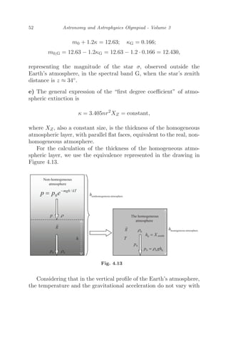
For the calculation of the thickness of the homogeneous atmo-
spheric layer, we use the equivalence represented in the drawing in
Figure 4.13.
Fig. 4.13
Considering that in the vertical profile of the Earth’s atmosphere,
the temperature and the gravitational acceleration do not vary with
64.
Two Astronomical Observatorieson an Island 53
the altitude, h, the density of the atmospheric air, due to the action
of the terrestrial gravitational forces, is given by the law
ρ = ρ0e−m1gh/kT
,
where: ρ0 – atmospheric air density at sea level; m1 – average mass
of an “air molecule”; g = 9.81 m/s2 – gravitational acceleration; k –
Boltzmann’s constant; and T0 = 273.15 K – the absolute temperature
of the atmosphere.
If n is the volume concentration of “air molecules”, it results that:
ρ =
m
V
=
m1N
V
= m1n,
where m1 is the mass of an “air molecule”;
ρ0 =
m0
V
=
m1N0
V
= m1n0;
ρ = ρ0e−m1gh/kT
;
m1n = m1n0e−m1gh/kT
; n = n0e−m1gh/kT0
;
p = nkT; p0 = n0kT;
p
kT
=
p0
kT
e−m1gh/kT
;
p = p0e−m1gh/kT
,
representing the barometric formula for the variation of atmospheric
pressure with altitude;
p0 = ρ0gh0; p0 = 1.013 · 105 N
m2
;
ρ0 =
p0
gh0
=
1.013 · 105
9.81 · 8 · 103
kg
m3
= 1.29
kg
m3
,
representing the air density in the homogeneous atmosphere equiva-
lent to the real, inhomogeneous atmosphere.
65.
54 Astronomy andAstrophysics Olympiad - Volume 3
Fig. 4.14
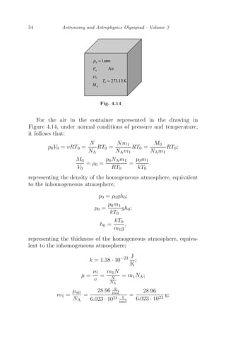
For the air in the container represented in the drawing in
Figure 4.14, under normal conditions of pressure and temperature,
it follows that:
p0V0 = vRT0 =
N
NA
RT0 =
Nm1
NAm1
RT0 =
M0
NAm1
RT0;
M0
V0
= ρ0 =
p0NAm1
RT0
=
p0m1
kT0
,
representing the density of the homogeneous atmosphere, equivalent
to the inhomogeneous atmosphere;
p0 = ρ0gh0;
p0 =
p0m1
kT0
gh0;
h0 =
kT0
m1g
,
representing the thickness of the homogeneous atmosphere, equiva-
lent to the inhomogeneous atmosphere;
k = 1.38 · 10−23 J
K
;
μ =
m
v
=
m1N
N
NA
= m1NA;
m1 =
μair
NA
=
28.96 g
mol
6.023 · 1023 1
mol
=
28.96
6.023 · 1023
g;
66.
Two Astronomical Observatorieson an Island 55
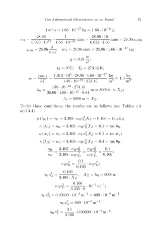
1 amu = 1.66 · 10−27
kg = 1.66 · 10−24
g;
m1 =
28.96
6.023 · 1023
·
1
1.66 · 10−24
amu =
28.96 · 10
6.023 · 1.66
amu = 28.96 amu;
μair = 28.96
g
mol
; m1 = 28.96 amu = 28.96 · 1.66 · 10−27
kg;
g = 9.81
m
s2
;
t0 = 0◦
C; T0 = 273.15 K;
ρ0 =
p0m1
kT
=
1.013 · 105 · 28.96 · 1.66 · 10−27
1.38 · 10−23 · 273.15
kg
m3
≈ 1.3
kg
m3
;
h0 =
1.38 · 10−23 · 273.15
28.96 · 1.66 · 10−27 · 9.81
m ≈ 8000 m = XZ;
h0 = 8000 m = XZ.
Under these conditions, the results are as follows (see Tables 4.3
and 4.4)
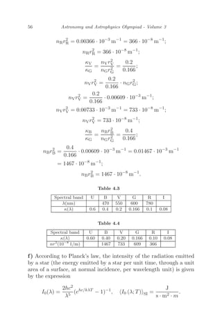
κ (λG) = κG = 3.405 · nGr2
GXZ = 0.166 = tan θG;
κ (λR) = κR = 3.405 · nRr2
RXZ = 0.1 = tan θR;
κ (λV) = κV = 3.405 · nVr2
VXZ = 0.2 = tan θV;
κ (λB) = κB = 3.405 · nBr2
BXZ = 0.4 = tan θB;
κR
κG
=
3.405 · nRr2
R
3.405 · nGr2
G
=
nRr2
R
nGr2
G
=
0.1
0.166
;
nRr2
R =
0.1
0.166
· nGr2
G;
nGr2
G =
0.166
3.405 · XZ
; XZ = h0 = 8000 m;
nGr2
G =
0.166
3.405 · 8
· 10−3
m−1
;
nGr2
G = 0.00609 · 10−3
m−1
= 609 · 10−8
m−1
;
nGr2
G = 609 · 10−8
m−1
;
nRr2
R =
0.1
0.166
· 0.00609 · 10−3
m−1
;
67.
56 Astronomy andAstrophysics Olympiad - Volume 3
nRr2
R = 0.00366 · 10−3
m−1
= 366 · 10−8
m−1
;
nRr2
R = 366 · 10−8
m−1
;
κV
κG
=
nVr2
V
nGr2
G
=
0.2
0.166
;
nVr2
V =
0.2
0.166
· nGr2
G;
nVr2
V =
0.2
0.166
· 0.00609 · 10−3
m−1
;
nVr2
V = 0.00733 · 10−3
m−1
= 733 · 10−8
m−1
;
nVr2
V = 733 · 10−8
m−1
;
κB
κG
=
nBr2
B
nGr2
G
=
0.4
0.166
;
nBr2
B =
0.4
0.166
· 0.00609 · 10−3
m−1
= 0.01467 · 10−3
m−1
= 1467 · 10−8
m−1
;
nBr2
B = 1467 · 10−8
m−1
.
Table 4.3
Spectral band U B V G R I
λ(nm) 470 550 600 780
κ(λ) 0.6 0.4 0.2 0.166 0.1 0.08
Table 4.4
Spectral band U B V G R I
κ(λ) 0.60 0.40 0.20 0.166 0.10 0.08
nr2
(10−8
1/m) 1467 733 609 366
f) According to Planck’s law, the intensity of the radiation emitted
by a star (the energy emitted by a star per unit time, through a unit
area of a surface, at normal incidence, per wavelength unit) is given
by the expression
I0(λ) =
2hc2
λ5
(ehc/kλT
− 1)−1
, I0 (λ; T)SI =
J
s · m2 · m
.
68.
Two Astronomical Observatorieson an Island 57
From this, particularizing for each of the visible spectral bands, it
results that (see Table 4.5):
I0,G(λG) =
2hc2
λ5
G
(ehc/kλGT
− 1)−1
; λG = 600 nm;
tan θG = κG = 0.166;
k = 1.38 · 10−23 J
K
; h = 6.625 · 10−34
Js; T = 6000 K;
hc
kλGT
=
6.625 · 10−34 J · s · 3 · 108 m
s
1.38 · 10−23 J
K · 600 · 10−9 m · 6000 K
≈ 0.4;
I0,R(λR) =
2hc2
λ5
R
(ehc/kλRT
− 1)−1
; λR = 780 nm;
hc
kλRT
=
6.625 · 10−34 J · s · 3 · 108 m
s
1.38 · 10−23 J
K · 780 · 10−9 m · 6000 K
≈ 0.3;
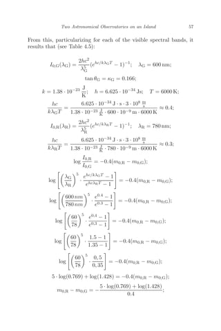
log
I0,R
I0,G
= −0.4(m0,R − m0,G);
log
λG
λR
5
·
ehc/kλGT − 1
ehcλRT − 1
= −0.4(m0,R − m0,G);
log
600 nm
780 nm
5
·
e0.4 − 1
e0.3 − 1
= −0.4(m0,R − m0,G);
log
60
78
5
·
e0,4 − 1
e0,3 − 1
= −0.4(m0,R − m0,G);
log
60
78
5
·
1.5 − 1
1.35 − 1
= −0.4(m0,R − m0,G);
log
60
78
5
·
0, 5
0, 35
= −0.4(m0,R − m0,G);
5 · log(0.769) + log(1.428) = −0.4(m0,R − m0,G);
m0,R − m0,G = −
5 · log(0.769) + log(1.428)
0.4
;
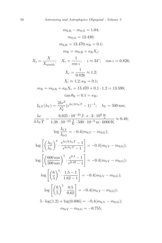
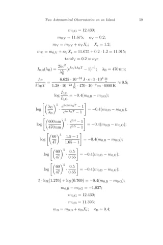
60 Astronomy andAstrophysics Olympiad - Volume 3
Xr = 1.2; mB = m0,B + κBXr = 11.393 + 0.4 · 1.2 = 11.873;
tan θB = 0.4 = κB;
m0,G = 12.430;
mG = m0,G + κGXr; κG = 0.166;
Xr = 1.2; mG = m0,G + κGXr = 12.430 + 0.166 · 1.2 = 12.629;
tan θG = 0.166 = κG.
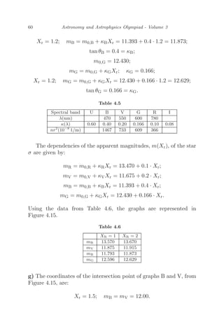
Table 4.5
Spectral band U B V G R I
λ(nm) 470 550 600 780
κ(λ) 0.60 0.40 0.20 0.166 0.10 0.08
nr2
(10−8
1/m) 1467 733 609 366
The dependencies of the apparent magnitudes, m(Xr), of the star
σ are given by:
mR = m0,R + κRXr = 13.470 + 0.1 · Xr;
mV = m0,V + κVXr = 11.675 + 0.2 · Xr;
mB = m0,B + κBXr = 11.393 + 0.4 · Xr;
mG = m0,G + κGXr = 12.430 + 0.166 · Xr.
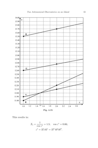
Using the data from Table 4.6, the graphs are represented in
Figure 4.15.
Table 4.6
XR = 1 XR = 2
mR 13.570 13.670
mV 11.875 11.915
mB 11.793 11.873
mG 12.596 12.629
g) The coordinates of the intersection point of graphs B and V, from
Figure 4.15, are:
Xr = 1.5; mB = mV = 12.00.
72.
Two Astronomical Observatorieson an Island 61
Fig. 4.15
This results in:
Xr =
1
cos z∗
= 1.5; cos z∗
= 0.66;
z∗
= 37.83◦
= 37◦
49
48
.
73.
62 Astronomy andAstrophysics Olympiad - Volume 3
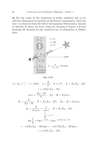
h) For the study of the extinction of stellar radiation due to its
selective absorption by particles in the Earth’s atmosphere, when the
star σ is observed from the OA-2 Astronomical Observatory, located
at altitude H above sea level, using the drawing in Figure 4.16 and
knowing the formula for the empirical law of absorption, it follows
that:
Fig. 4.16
I = I0 · e−τ
; τ = nSX; n =
N
V
; S = πr2
; X = Xr(XZ − H);
τ = nSXr(XZ − H);
cos z =
XZ − H
X
; XZ − H = X cos z;
Xr =
X
XZ − H
; X = Xr(XZ − H); XZ − H = X cos z;
Xr =
X
X cos z
=
1
cos z
; X = Xr(XZ − H);
I
I0
= e−τ
;
log
I
I0
= log e−nSX
= log e−nSXr(XZ−H)
= −nSXr(XZ − H) log e = −nπr2
Xr(XZ − R) log e;
τ = nSXr(XZ − H);
74.
Two Astronomical Observatorieson an Island 63
π = 3.14; e = 2.718; log e = log(2.719) = 0.434;
log
I
I0
= −0.434nπ r2
Xr(XZ − H) = −0.434 · 3.14nr2
Xr(XZ − H);
log
I
I0
= −1.362nr2
(XZ − H)Xr.
On the other hand, according to Pogson’s formula, it follows that:
log
I
I0
= −0.4(m − m0); (m − m0) = −2.5 · log
I
I0
,
where m0 is the apparent magnitude of the star, seen from outside the
atmosphere (not affected by the phenomenon of atmospheric extinc-
tion) and m is the apparent magnitude of the star for the observer
(affected by the phenomenon of atmospheric extinction);
m − m0 = −2.5 · log
I
I0
= 2.5 · 1.362nr2
(XZ − H)Xr;
m − m0 = 3.405nr2
(XZ − H)Xr;
κOA-2 = 3.405nr2
(XZ − H) = constant.
The above is a combination of constant quantities (n, r, XZ, H),
called the “coefficient of the first degree” of atmospheric extinction,
at the OA-2 Astronomical Observatory, so that:
κOA-2 = 3.405nr2
XZ − 3.405nr2
H;
m − m0 = κOA-2Xr;
m = m0 + κOA-2Xr.
This proves that the magnitude of the star for the observer at the
altitude H, OA-2, after the extinction of the light in the atmosphere,
is a function of the parameter
Xr = “air mass”,
whose physical meaning is that of the relative distance traveled by
light from entering the Earth’s atmosphere to the observer:
Xr =
X
XZ − H
,
75.
64 Astronomy andAstrophysics Olympiad - Volume 3
that is, the ratio of the distance traveled by starlight through the
atmosphere to the observer when the star is at some position in the
sky, to the distance traveled by starlight through the atmosphere to
the observer when the star is at the observer’s zenith;
Xr ≥ 1;
m(Xr) = m0 + κOA-2Xr; tan θOA-2 = κOA-2.
This results in:
m − m0 = −2.5 · log I
I0
= 2.5 · 1.362nr2(XZ − H)Xr;
−2.5 · log I
I0
= 3.405nr2(XZ − H)Xr = κOA-2Xr;
−2.5 · log I
I0
= (3.405nr2XZ − 3.405nr2H)Xr = κOA-2Xr;
(3.405nr2XZ − 3.405nr2H) = κOA-2 = tan θOA-2.
Thus, in the band of yellow radiation, we obtain:
−2.5 · log
I
I0
= (3.405nGr2
GXZ − 3.405nGr2
GH)Xr = κOA-2,GXr;
(3.405nGr2
GXZ − 3.405nGr2
GH) = κOA-2,G,
where
nGr2
G = 609 · 10−8
m−1
, XZ = 8000 m, H = 500 m.
Thus:
−2.5 · log
I
I0
= 0.15 · Xr = κOA-2,GXr;
κOA-2,G = 0.15 = tan θOA-2,G;
−2.5 · log
I
I0
= 0.15Xr;
−2.5 · log
I
I0
= 0.15Xr; Xr =
1
cos z
;
−2.5 · log
I
I0
=
0.15
cos z
=
0.15
cos 34◦
=
0.15
0.829
;
76.
Two Astronomical Observatorieson an Island 65
log
I
I0
= −
0.15
0.829 · 2.5
= −0.07;
η =
I
I0
= 0.85; I = 0.85 · I0.
Additionally:
3.405nGr2
GXZ − 3.405nGr2
GH = κOA-2,G = tan θOA-2,G;
3.405nGr2
GXZ = tan θOA-1,G = tan θG = κG = 0.166;
nGr2
G = 609 · 10−8
m−1
; H = 500 m;
tan θOA-1 − 3.405nGr2
GH = tan θOA-2,G;
tan θOA-2,G = tan θOA-1 − 3.405nGr2
GH;
tan θOA-2,G tan θOA-1,G;
θOA-2,G θOA-1;
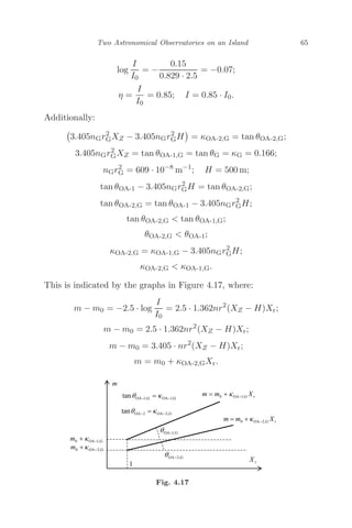
κOA-2,G = κOA-1,G − 3.405nGr2
GH;
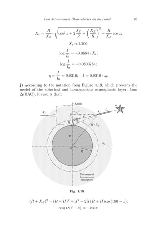
κOA-2,G κOA-1,G.
This is indicated by the graphs in Figure 4.17, where:
m − m0 = −2.5 · log
I
I0
= 2.5 · 1.362nr2
(XZ − H)Xr;
m − m0 = 2.5 · 1.362nr2
(XZ − H)Xr;
m − m0 = 3.405 · nr2
(XZ − H)Xr;
m = m0 + κOA-2,GXr.
Fig. 4.17
77.
66 Astronomy andAstrophysics Olympiad - Volume 3
Fig. 4.18
i) In accordance with the notation in Figure 4.18, where the model of
the spherical and homogeneous atmospheric layer is presented, from
Δ(OAB), it follows that:
(R + X cos z)2
+ (X sin z)2
= (R + XZ)2
;
R2
+ 2RX cos z + X2
cos2
z + X2
sin2
z = R2
+ 2RXZ + X2
Z;
2RX cos z + X2
= 2RXZ + X2
Z;
X2
+ 2R cos z · X − XZ (2R + XZ) = 0;
X = R2 cos2 z + XZ (2R + XZ) − R cos z;
Xr =
X
XZ
=
R2 cos2 z + XZ (2R + XZ) − R cos z
XZ
;
78.
Two Astronomical Observatorieson an Island 67
Xr =
R2 cos2 z + XZ
2R2
R + XZ
R2
R2
− R cos z
XZ
;
Xr =
R2 cos2 z + R2
2XZ
R +
X2
Z
R2
− R cos z
XZ
;
Xr =
R · cos2 z +
2XZ
R +
X2
Z
R2
− R cos z
XZ
;
Xr =
R
XZ
· cos2 z + 2
XZ
R
+
XZ
R
2
−
R
XZ
cos z;
I = I0 · e−τ
; τ = nSX; Xr =
X
XZ
; X = XZXr;
I
I0
= e−τ
; log
I
I0
= log e−nSX
= log e−nSXZXr
= −nSXZXr log e;
e = 2.718;
log
I
I0
= −0.434nπ r2
XZXr = −0.434 · 3, 14nr2
XZXr
= −1.362nr2
XZXr;
log
I
I0
= −0.4(m − m0);
m − m0 = −2.5 · log
I
I0
= 2.5 · 1.362nr2
XZXr = 3.405nr2
XZXr;
−2.5 · log
I
I0
= 3.405nr2
XZXr;
κ = 3.405nr2
XZ; −2.5 · log
I
I0
= κXr;
log
I
I0
= −1.362 · nr2
XZXr;
κ = 3.405nr2
XZ = constant,
79.
68 Astronomy andAstrophysics Olympiad - Volume 3
being a combination of constant quantities (n, r, XZ), called the
“coefficient of the first degree” of atmospheric extinction.
Using the graph represented in Figure 4.12, the validity of which
is maintained in this case as well, it results that:
tan θ = κ =
Δm
ΔXr
=
0.05
0.3
≈ 0.166;
−2.5 · log
I
I0
= κXr; −2.5 · log
I
I0
= 0.166 · Xr;
log
I
I0
= −0.0664 · Xr;
Xr =
R
XZ
· cos2 z + 2
XZ
R
+
XZ
R
2
−
R
XZ
cos z;
log
I
I0
= −0.0664 ·
⎡
⎣ R
XZ
· cos2 z + 2
XZ
R
+
XZ
R
2
−
R
XZ
cos z
⎤
⎦;
XZ = 8000 m; R = 6370 km; z = 34◦
; cos z = 0.829;
R
XZ
= 796.25;
XZ
R
= 0.001255886; 2
XZ
R
= 0.002511773;
XZ
R
2
= 0.000001577; cos2
z = 0.687241;
cos2 z + 2
XZ
R
+
XZ
R
2
= 0.830514509;
R
XZ
· cos2 z + 2
XZ
R
+
XZ
R
2
= 661.297178;
R
XZ
cos z = 660.09125;
Xr =
⎡
⎣ R
XZ
· cos2 z + 2
XZ
R
+
XZ
R
2
−
R
XZ
cos z
⎤
⎦ = 1.205928;
80.
Two Astronomical Observatorieson an Island 69
Xr =
R
XZ
· cos2 z + 2
XZ
R
+
XZ
R
2
−
R
XZ
cos z;
Xr ≈ 1.206;
log
I
I0
= −0.0664 · Xr;
log
I
I0
= −0.0800784;
η =
I
I0
= 0.8316; I = 0.8316 · I0.
j) According to the notation from Figure 4.19, which presents the
model of the spherical and homogeneous atmospheric layer, from
Δ(OAC), it results that:
Fig. 4.19
(R + XZ)2
= (R + H)2
+ X2
− 2X(R + H) cos(180 − z);
cos(180◦
− z) = −cosz;
81.
70 Astronomy andAstrophysics Olympiad - Volume 3
(R + XZ)2
= (R + H)2
+ X2
+ 2X(R + H) cos z;
X2
+ 2(R + H) cos z · X − 2RXZ − X2
Z + 2RH + H2
= 0;
X = −(R + H) cos z ±
(R + H)2 cos2 z + 2RXZ + X2
Z − 2RH − H2;
X = −(R + H) cos z ±
(R + H)2 cos2 z + 2R(XZ − H) + X2
Z − H2;
X = −(R + H) cos z +
(R + H)2 cos2 z + 2R(XZ − H) + X2
Z − H2;
Xr =
X
XZ − H
;
Xr =
(R + H)2 cos2 z + 2R(XZ − H) + X2
Z − H2 − (R + H) cos z
XZ − H
;
Xr =
1
XZ − H
·
(R + H)2 cos2 z + 2R(XZ − H) + X2
Z − H2
−
R + H
XZ − H
cos z;
Xr =
R + H
XZ − H
2
cos2 z +
2R(XZ − H)
(XZ − H)2
+
X2
Z − H2
(XZ − H)2
−
R + H
XZ − H
cos z;
Xr =
R + H
XZ − H
2
cos2 z +
2R
(XZ − H)
+
(XZ − H)(XZ + H)
(XZ − H)2
−
R + H
XZ − H
cos z;
Xr =
R + H
XZ − H
2
cos2 z +
2R
(XZ − H)
+
(XZ + H)
(XZ − H)
−
R + H
XZ − H
cos z;
XZ = 8000 m; R = 6370 km; z = 34◦
; cos z = 0.829; H = 500 m;
R + H
XZ − H
= 849.4;
2R
XZ − H
= 1698.666;
XZ + H
XZ − H
= 1.133;
Xr = 1.206950;
82.
Two Astronomical Observatorieson an Island 71
Xr ≈ 1.207;
log
I
I0
= −0.0664 · Xr;
log
I
I0
≈ −0.0801448;
η =
I
I0
= 0.8315; I = 0.8315 · I0.
83.
This page intentionallyleft blank
This page intentionally left blank
84.
Problem 5
Moons ofJupiter
Given the relevant data for Jupiter’s four moons (Io, Europa,
Ganymede, and Callisto), two astronomers plotted the graphs shown
in Figures 5.1 and 5.2, each of which represents the dependence graph
log |T(s)| = f(log |a(m)|), where: |T(s)| – the numerical value of the
period of each month expressed in seconds; |a(m)| – the numerical
value of the average distance between Jupiter and any of its moons,
expressed in meters.
Fig. 5.1
73
85.
74 Astronomy andAstrophysics Olympiad - Volume 3
Fig. 5.2
a) Between the graphic variants represented in Figures 5.1 and
5.2, identify the correct version of the dependence log |T(s)| =
f(log |a(m)|), valid for the four moons of Jupiter: Io, Europa,
Ganymede, and Callisto.
b) Determine the mass of Jupiter, knowing the value of the gravita-
tional constant, K = 6.673 · 10−11 Nm2
kg−2
.
Jupiter’s mass is known to be much greater than the mass of any
of its moons.
Solution
a) Kepler’s third law is written for Jupiter and any of its moons as
follows:
T2
=
4π2
K(M + m)
· a3
.
This results in:
M m;
T2
=
4π2
KM
· a3
;
86.
Moons of Jupiter75
2 log T = log
4π2
K
− log M + 3 log a;
log T =
1
2
· log
4π2
K
−
1
2
· log M +
3
2
· log a;
log T =
3
2
· log a +
1
2
· log
4π2
K
−
1
2
· log M;
log T = y; log a = x;
m =
3
2
;
1
2
· log
4π2
K
−
1
2
· log M = b;
y = mx + b,
representing the equation of a straight line, where m = 3
2 = 1.5
indicates the slope of the straight line, which is also calculated from
each graph. This results in:
(Fig. 5.1) m = 1.5;
(Fig. 5.2) m = 1.6.
So, we identify the graphic representation in Figure 5.1 as correct.
b) With the notation and numerical values presented on the system
of axes in Figure 5.3, it results that:
.
.
Fig. 5.3
This page intentionallyleft blank
This page intentionally left blank
90.
Problem 6
A CometAround the Sun
The rotation period of a comet around the Sun is Tc = 76 years,
and the minimum distance of the comet from the Sun is rc,min =
1.8 · 108 km. Determine the maximum distance between the comet
and the Sun, rc,max. Given: the radius of the Earth’s circular orbit
around the Sun, RE = 1.5·108 km; the period of rotation of the Earth
around the Sun, TE = 1 year.
Solution
According to Kepler’s third law, it follows that:
rc,min + rc,max = 2ac;
T2
E =
4π2
KMS
R3
E; T2
c =
4π2
KMS
a3
c;
rc,max = 2RE · 3
T2
c
T2
E
− rc,min.
79
91.
This page intentionallyleft blank
This page intentionally left blank
92.
Problem 7
Visible CircumpolarStars
It is commonly believed that the number of stars visible to the naked
eye in the entire sky is N = 6000 stars. Estimate the number of
circumpolar stars visible to the naked eye, Nc, if the observer is
placed at the angular distances:
a) Δα = 1◦, towards the North Pole;
b) Δα = 1◦, towards the Equator, towards the north.
Solution
a) For an observer located in the center O of the topocentric celestial
sphere, at latitude ϕ and at sea level (zero altitude), all the stars
represented in the drawing in Figure 7.1 appear as circumpolar stars.
Their diurnal parallels, parallels to the celestial equator, lie above
the true horizon of the place (N0S0). The star σ0 is at the limit of
circumpolarity because its diurnal parallel touches the true horizon
of the place, at the point N0, but remains above it. Star σ0 is a
marginally circumpolar star.
The variant presented does not take into account the refraction
of light coming from the star, crossing the Earth’s atmosphere.
For this observer, from the isosceles triangle Oσ0N0, it results
that:
δ0,min + 90◦
+ (ϕ − δmin) = 180◦
;
δ0,min = 90◦
− ϕ.
81
93.
82 Astronomy andAstrophysics Olympiad - Volume 3
Fig. 7.1
Under the conditions of the problem, if the observer is near the
geographic North Pole, as indicated by the drawing in Figure 7.2, the
angular distance means that the observer is at an observation point
with the latitude ϕ = 89◦. As a result, for this observer, the star σ0
with the declination δ0,min = 90◦ − ϕ = 1◦ is at the limit of circum-
polarity. Thus, for this observer, the stars above the celestial equator
contained in the equatorial belt of angular width Δθ = δ0,min = 1◦
will not be visible circumpolar stars. They will be rising and setting
stars. So will the stars included in the equatorial belt below the equa-
tor to the diurnal parallel of S0. The stars below the diurnal parallel
of S0 are circumpolar stars from the southern celestial hemisphere,
invisible to the considered observer.
As a result of these clarifications, for the observer located in the
Northern Hemisphere at the latitude ϕ = 89◦, these stars will appear
as circumpolar stars visible to the naked eye. These stars are uni-
formly distributed on the surface of the spherical dome represented
in the drawing in Figure 7.3, where δ0,min = 1◦ and θ = 89◦.
We know that the surface area of the spherical dome and the
surface area of the sphere are:
Sdome = 2πRh = 2πR · R(1 − cos θ) = 4πR2
sin2 θ
2
;
Ssphere = 4πR2
.
94.
Visible Circumpolar Stars83
Fig. 7.2
Fig. 7.3
Assuming the uniform distribution of stars on the celestial sphere,
it follows that the ratio between the surface area of the dome on the
celestial sphere and the surface area of the entire celestial sphere is
equal to the ratio between the number of stars on the dome and the
95.
84 Astronomy andAstrophysics Olympiad - Volume 3
number of stars on the entire celestial sphere:
Nstars dome
Nstars sphere
=
Sdome
Ssphere
.
So, it follows that:
Nstars dome
Nstars sphere
=
4πR2 sin2 θ
2
4πR2
= sin2 θ
2
;
Nstars dome
Nstars sphere
= sin2 θ
2
; Nstars dome = Nstars sphere · sin2 θ
2
;
Nstars dome = 6000 · sin2
(44.5◦
) ≈ 2947 stars.
For an observer located at the geographic North Pole (ϕ = +90◦),
the celestial North Pole, P, is confused with the zenith, Z, so that
the Earth’s axis, PP, is confused with the local vertical, ZZ, and the
plane of the celestial equator, QQ, is confused with the plane of the
astronomical horizon, NS, as indicated by the drawing in Figure 7.4.
The observer on
the geographic
North Pole
Fig. 7.4
96.
Visible Circumpolar Stars85
Under these conditions, the observer at the geographic North Pole
appreciates that the diurnal celestial parallels of the stars are paral-
lel both to the celestial equator and to the true horizon so that, in
relation to the observer, all the stars in the northern celestial hemi-
sphere (δ 0) are stars without sunset (always visible), and the stars
in the southern celestial hemisphere (δ 0) are stars without sunrise
(always invisible).
The number of circumpolar stars (without sunset) visible to the
naked eye if the observer were right at the geographic North Pole
would be half of the total number (6000) of stars visible in the entire
sky to the naked eye, that is, 3000 stars. These are the stars whose
declination is δ 0.
b) For the observer at the latitude ϕ = Δα = 1◦, as indicated in the
drawing in Figure 7.5, the star σ0, at the limit of circumpolarity, is
at the angular distance Δα = 1◦ from the celestial North Pole, P.
Fig. 7.5
97.
86 Astronomy andAstrophysics Olympiad - Volume 3
Fig. 7.6
As a result of these clarifications, for the observer located in the
Northern Hemisphere at latitude ϕ = 1◦, these stars will appear as
circumpolar stars visible to the naked eye, uniformly distributed on
the surface of the spherical dome, with height h, represented in the
drawing in Figure 7.6, where δ0,min = 89◦ and Δα = 1◦.
We know that the surface area of the spherical dome and the
surface area of the sphere are:
Sdome = 2πRh = 2πR · R(1 − cos Δα) = 4πR2
sin2 Δα
2
;
sin Δα ≈ Δα;
Sdome ≈ 4πR2
·
(Δα)2
4
= πR2
· (Δα)2
;
Ssphere = 4πR2
.
Assuming the uniform distribution of stars on the celestial sphere,
it follows that the ratio between the surface area of the dome on the
celestial sphere and the surface area of the entire celestial sphere is
equal to the ratio between the number of stars on the dome and the
number of stars on the entire celestial sphere:
Nstars dome
Nstars sphere
=
Sdome
Ssphere
.
98.
Visible Circumpolar Stars87
So, it follows that:
Nstars dome
Nstars sphere
=
πR2 · (Δα)2
4πR2
=
1
4
· (Δα)2
;
Nstars dome =
Nstars sphere
4
· (Δα)2
;
Nstars dome ≈ 0.45,
representing the number of circumpolar stars visible to the observer
at latitude ϕ = 1◦.
Being a sub-unit fraction, the result is unacceptable. It means
that looking with the naked eye from the specified position, none of
the stars in the sky will be appreciated as a visible circumpolar star!
In particular, for an observer located right on the terrestrial Equa-
tor (ϕ = 0), the north celestial pole, P, is on the horizon, at the
north celestial cardinal point, N, and the south celestial pole, P, is
on the horizon at the south celestial cardinal point, S, as indicated
by the drawing in Figure 7.7. The plane of the celestial equator is
Fig. 7.7
99.
88 Astronomy andAstrophysics Olympiad - Volume 3
perpendicular to the plane of the true horizon of the place, inter-
secting it according to the direction of the celestial cardinal points
east–west, passing through Z and Z.
Under these conditions, the observer on the terrestrial Equator
appreciates that the diurnal celestial parallels of the stars are circles
parallel to the celestial equator, perpendicular to the plane of the
true horizon, so that, relative to the observer, all the stars have risen
(on the NES sector of the true horizon) and set (on the SWN sector
of the true horizon).
Half of the length of the diurnal parallel of each star is above the
true horizon, and the other half is below the true horizon, so that
the duration of visibility of each star is equal to the duration of its
invisibility (12 h). For this observer there are no visible circumpo-
lar stars.
100.
Problem 8
Cepheid Period
Cepheidsare stars whose volumes are radially variable, through
alternate compressions and dilations (Cepheids keep their spheri-
cal shapes), with short periods, P, from 1 to 130 days, which causes
periodic variations in their brightness, materializing as variations in
their apparent magnitudes, which can reach Δm = 2m.
During the radial fluctuations of a Cepheid, it remains a homo-
geneous sphere (with constant density, ρ). In addition, we consider
that the temperature and the mass of the Cepheid remain constant,
T and μ, respectively.
a) Determine the period of the radial variation of the Cepheid’s
volume, P, knowing the Cepheid’s density, ρ, and the gravitational
attraction constant, K.
b) Determine the apparent magnitude, m, of the Cepheid.
It is known that, for the homogeneous differential equation
d2R
dt2
− q · R = 0,
where R = R(t) is the radius of the Cepheid at a given moment, and
q is a constant quantity, the general solution is
R(t) = a · cos(
√
q · t) + b · sin(
√
q · t),
where a and b are integration constants. For this expression, with P
being the period of the radial variation of the Cepheid’s volume, it
89