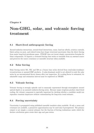
CFR-RF v1.1: A Formal Framework for Climate Forcing and Response Research
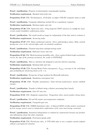
Comprehensive research standard for evaluating climate change causation through energy balance, forcing models, and falsifiable hypotheses from 1750 to 2031 with rigorous validation and uncertainty analysis.
CFR-RF v1.1: A Formal Framework for Climate Forcing and Response Research
1.
CFR-RF v1.1
Climate Forcing→ Response Research Framework
Full Research Standard and Formal Mathematical Edition
Formal attribution, falsification, physical consistency, out-of-sample validation, and
prospective testing architecture
System architect: Vadym Tsinderhoz
Document date: 24 August 2026
Language: English
Status: RESEARCH STANDARD PROPOSAL / PRE-RESULT
Evidence mode: Historical pseudo-OOS + prospective-capable
Target execution horizon: 1750–2031
Status notice. This document defines a falsifiable research architecture. It is not an IPCC,
ISO, governmental, regulatory, clinical, or legal standard. It does not assume in advance that
anthropogenic, natural, solar, internal-variability, or observational-bias explanations are correct.
Mathematical statements are separated from empirical climate claims. Empirical conclusions
require execution on locked data under the frozen protocol. Historical data available before 24
August 2026 cannot constitute genuinely unseen prospective evidence.
2.
Abstract
CFR-RF is aformal research framework for adversarial comparison of competing explanations
of observed climate change. Its central question is not whether a single time series correlates
with atmospheric carbon dioxide, but which pre-registered causal architecture can simultaneously
account for the evolution of surface temperature, ocean heat storage, top-of-atmosphere energy
imbalance, and independent spatial or vertical fingerprints while satisfying energy conservation,
measurement uncertainty, model-complexity constraints, data-lineage rules, and out-of-sample
prediction requirements.
The framework registers nine principal model classes, M0–M8, ranging from null/internal sta-
tistical benchmarks to natural-only, solar-dominant, bounded observational-bias, greenhouse-gas,
all-anthropogenic, and full anthropogenic-plus-natural physical models. It combines exact effective-
radiative-forcing equations for major well-mixed greenhouse gases, an energy-conserving two-layer
energy-balance model, regularized detection-and-attribution regression, covariance-aware errors-
in-variables sensitivity analysis, forcing-uncertainty propagation, blocked resampling for serially
correlated time series, multi-dataset transfer tests, and ten mandatory decision gates G0–G9.
The architecture is explicitly falsifiable. Passing a warming gate does not by itself establish anthro-
pogenic causation. Failure of an anthropogenic model does not automatically validate a solar or
internal-variability model. A natural-only alternative must independently satisfy its own predictive,
energetic, fingerprint, uncertainty, and transfer requirements. Conversely, if anthropogenic-plus-
natural models consistently outperform natural-only competitors out of sample, survive greenhouse-
gas ablation, reproduce non-temperature energy endpoints, remain stable across forcing and co-
variance uncertainty, transfer to independent observational products, and continue to perform in
genuinely post-lock observations, the framework yields progressively stronger support for anthro-
pogenic attribution within its stated domain.
The document provides definitions, assumptions, proofs, exact equations, numerical verification
vectors, a causal directed acyclic graph, a data firewall spanning 1750–2031, model specifications,
a data-version and SHA-256 policy, a failure-mode-and-effects analysis, requirements traceability,
synthetic positive and negative controls, a reference software implementation, frozen configuration,
and executable unit tests. Current published climate measurements are used only as external context
and verification inputs; they are not presented as results generated by CFR-RF unless explicitly
identified as a framework calculation.
1
3.
Executive scientific statement
Thestrongest scientific use of CFR-RF is as a controlled attempt to make competing climate-
causation hypotheses lose under conditions declared before the decisive evaluation. A hypothesis
that cannot lose is not suitable for this framework. A hypothesis that fits global mean temperature
but violates the planetary energy budget cannot achieve the strongest status. A hypothesis that
relies on a data-product revision or post-hoc tuning after test access must be classified as Invalid
for that version. A hypothesis that appears favorable only under one forcing reconstruction or one
covariance treatment is classified as unstable unless its sensitivity behavior was pre-registered.
As of the document date, established assessments and updated peer-reviewed indicators provide strong
prior evidence that recent global warming is predominantly human-induced. For example, the 2026
Indicators of Global Climate Change 2025 assessment reports observed warming of approximately
1.26 °C for 2016–2025 relative to 1850–1900 and assessed human-induced warming of approximately
1.24 °C for the same decade, with published uncertainty ranges; for 2025 it reports observed warming
of approximately 1.39 °C and assessed human-induced warming of approximately 1.37 °C. These
values are context, not CFR-RF output. The framework is designed so that these conclusions
remain challengeable by a pre-specified, physically coherent, out-of-sample alternative rather than
by selective correlation or retrospective model rescue.[5]
2
List of Figures
3.1CFR-RF causal attribution graph. Arrows indicate pre-specified causal or observation
pathways; they do not represent fitted effect sizes. . . . . . . . . . . . . . . . . . . . 21
7.1 Published NOAA 2024 long-lived-GHG forcing context. The first three bars are
calculated by the CFR-RF frozen equations from NOAA-reported 2024 concentrations;
the residual bar is the difference to NOAA’s reported total long-lived-GHG ERF. . . 29
9.1 Primary two-layer energy-balance model used for the global physical branch. . . . . 31
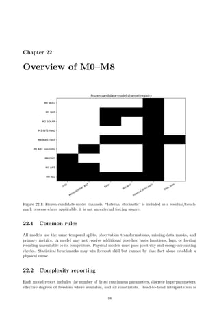
22.1 Frozen candidate-model channels. “Internal stochastic” is included as a residual/bench-
mark process where applicable; it is not an external forcing source. . . . . . . . . . . 48
36.1 Published IGCC 2025 context. Error bars reproduce the published ranges cited in
the text. These values are external benchmarks, not CFR-RF analysis results. . . . . 64
43.1 Temporal firewall. The 2000–2025 blocks are historical pseudo-out-of-sample because
they were already public at specification time. . . . . . . . . . . . . . . . . . . . . . . 71
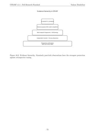
43.2 Evidence hierarchy. Genuinely post-lock observations have the strongest protection
against retrospective tuning. . . . . . . . . . . . . . . . . . . . . . . . . . . . . . . . . 72
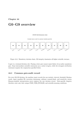
44.1 Mandatory decision chain. G0 integrity dominates all higher scientific statuses. . . . 74
14
Chapter 1
Purpose, researchobject, and scope
1.1 Purpose
CFR-RF is intended to convert a broad and politically contested question into a finite set of
testable research propositions. The framework asks which registered forcing-response architecture
best survives a common experimental and statistical protocol. It is designed for reproducibility,
adversarial comparison, and explicit negative results.
The object of study is the large-scale climate response to external radiative forcing and internal
variability over the instrumental and forcing-reconstruction era. The principal spatial scales are global
and broad zonal or regional aggregates. The principal temporal scales are annual to multi-decadal.
Weather attribution for individual events, local adaptation policy, integrated assessment economics,
and social-cost estimation are outside the primary confirmatory scope.
1.2 Central research question
For observation vector
Y(t, r) = {T, Hocean, NTOA, SST, SLR, ice, Ttrop, Tstrat, . . .},
which pre-registered causal model Mj provides the best physically admissible and transferable
prediction under locked forcing, covariance, uncertainty, and complexity rules?
1.3 Why temperature alone is insufficient
A surface-temperature series is an important but incomplete diagnostic. Internal variability can
temporarily alter surface temperature by exchanging energy among climate-system reservoirs. Ob-
servation pipelines can introduce correlated uncertainty. Different forcing combinations can produce
similar low-dimensional trajectories over finite periods. Therefore the strongest status requires at
least one direct or constrained energy-storage endpoint in addition to temperature and requires
consistency with physically expected fingerprints.
1.4 Status classes
Every top-level conclusion is classified as Pass, Fail, Invalid, or Unstable. Passmeans the
pre-registered criterion was satisfied. Failmeans the criterion was validly tested and not satisfied. In-
validmeans the evidence stream was compromised by a protocol, data, code, or physical-admissibility
17
19.
CFR-RF v1.1 -Full Research Standard Vadym Tsinderhoz
violation. Unstablemeans reasonable, pre-registered sensitivity treatments materially change the
result and no single confirmatory interpretation is justified.
18
20.
Chapter 2
Claim hierarchyand scientific meaning
2.1 C0: observed warming
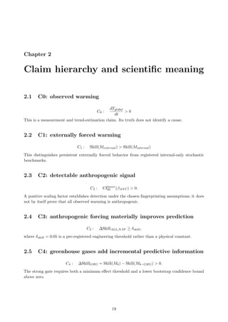
C0 :
dTglobal
dt
> 0
This is a measurement and trend-estimation claim. Its truth does not identify a cause.
2.2 C1: externally forced warming
C1 : Skill(Mexternal) > Skill(Minternal)
This distinguishes persistent externally forced behavior from registered internal-only stochastic
benchmarks.
2.3 C2: detectable anthropogenic signal
C2 : CIlower
95 (βANT ) > 0.
A positive scaling factor establishes detection under the chosen fingerprinting assumptions; it does
not by itself prove that all observed warming is anthropogenic.
2.4 C3: anthropogenic forcing materially improves prediction
C3 : ∆SkillALL,NAT ≥ δskill,
where δskill = 0.05 is a pre-registered engineering threshold rather than a physical constant.
2.5 C4: greenhouse gases add incremental predictive information
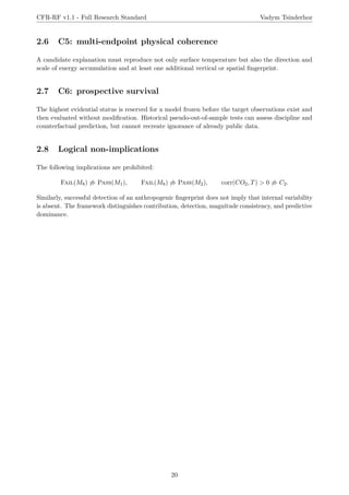
C4 : ∆SkillGHG = Skill(M8) − Skill(M8−GHG) > 0.
The strong gate requires both a minimum effect threshold and a lower bootstrap confidence bound
above zero.
19
21.
CFR-RF v1.1 -Full Research Standard Vadym Tsinderhoz
2.6 C5: multi-endpoint physical coherence
A candidate explanation must reproduce not only surface temperature but also the direction and
scale of energy accumulation and at least one additional vertical or spatial fingerprint.
2.7 C6: prospective survival
The highest evidential status is reserved for a model frozen before the target observations exist and
then evaluated without modification. Historical pseudo-out-of-sample tests can assess discipline and
counterfactual prediction, but cannot recreate ignorance of already public data.
2.8 Logical non-implications
The following implications are prohibited:
Fail(M8) ̸⇒ Pass(M1), Fail(M8) ̸⇒ Pass(M2), corr(CO2, T) > 0 ̸⇒ C2.
Similarly, successful detection of an anthropogenic fingerprint does not imply that internal variability
is absent. The framework distinguishes contribution, detection, magnitude consistency, and predictive
dominance.
20
22.
Chapter 3
Causal architecture
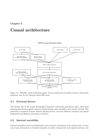
Figure3.1: CFR-RF causal attribution graph. Arrows indicate pre-specified causal or observation
pathways; they do not represent fitted effect sizes.
3.1 External drivers
The forcing side of the graph distinguishes long-lived well-mixed greenhouse gases, short-lived
anthropogenic forcing agents, land-use-related forcing, solar variability, and volcanic forcing. This
separation is required because distinct physical drivers can have different temporal and spatial
fingerprints and different uncertainty structures.
3.2 Internal variability
Internal variability enters as redistribution and stochastic modulation of the climate state. It may
cause large interannual or decadal anomalies in surface temperature and regional patterns, but
21
23.
CFR-RF v1.1 -Full Research Standard Vadym Tsinderhoz
an internal-only model is not permitted to create an unconstrained nonzero-mean external energy
source. A model that requires such a term changes class and must be re-registered.
3.3 Observation layer
Observation products are not treated as exact truth. Each product is represented as a measurement
operator applied to a latent state plus bias and random error. Product dependence must be recorded.
In particular, a derived radiation-budget product constrained using ocean heat storage cannot be
double-counted as independent confirmation of the same ocean heat constraint. NASA’s CERES
EBAF documentation explicitly describes an objective constrainment of global net TOA flux to be
consistent with Earth-system heat storage, which CFR-RF records in the provenance graph.[10]
22
24.
Chapter 4
Falsifiability, severity,and interpreta-
tion discipline
4.1 Predeclared defeat
For each strong claim, the framework states the conditions under which the claim fails. This
requirement prevents a moving-target interpretation in which every unexpected observation is
absorbed by an added parameter after test inspection.
4.2 Severity concept
A test has high scientific value when it had a substantial probability of exposing a false hypothesis.
CFR-RF increases severity through conjunction: a candidate must survive independent classes of
constraints including prediction, energy accounting, fingerprinting, uncertainty propagation, transfer,
and prospective evaluation. Passing one weakly informative test cannot compensate for failure of a
mandatory physical gate.
4.3 Negative results
A valid negative result is publication-worthy. The minimum report includes the frozen hypothesis,
gate value, confidence interval or diagnostic, data hashes, model parameters, sensitivity envelope,
and whether the result is Fail, Invalid, or Unstable. No failed mandatory gate may be omitted
from the confirmatory report.
4.4 What would materially challenge strong anthropogenic attri-
bution?
Within CFR-RF, a serious challenge requires more than a temporary temperature plateau or a
correlation with solar activity. A registered natural-only or internal model would need to match
or exceed the full model on held-out temperature while also explaining energy accumulation and
independent fingerprints with physically admissible parameters. In parallel, the anthropogenic
fingerprint would have to fail detection or transfer, and greenhouse-gas ablation would have to show
no robust loss of predictive skill. This is intentionally a demanding conjunction because the claim
being challenged is itself a multi-line-of-evidence causal claim.
23
25.
CFR-RF v1.1 -Full Research Standard Vadym Tsinderhoz
4.5 What would materially strengthen anthropogenic attribution?
Evidence strengthens when the anthropogenic-plus-natural model outperforms natural-only competi-
tors on frozen test periods, the anthropogenic scaling factor remains above zero under calibrated
uncertainty, removal of greenhouse-gas forcing degrades predictive skill, energy endpoints are consis-
tent, results transfer across observation products, forcing uncertainty does not reverse the conclusion,
and genuinely future observations remain within pre-registered predictive distributions.
24
Chapter 5
Earth’s energybudget
5.1 Global energy balance
At the top of the atmosphere, the global-mean climate system is governed by the difference between
absorbed solar radiation and outgoing radiation. IPCC AR6 expresses the perturbation energy
budget in terms of effective radiative forcing and temperature-dependent feedback. Using the
CFR-RF sign convention with a positive restoring coefficient λ > 0,
N(t) = F(t) − λTs(t),
where N > 0 denotes net downward energy accumulation. This is equivalent to the common IPCC
form ∆N = ∆F + α∆T when λ = −α.[2]
5.2 Energy-to-heat conversion
Using Earth radius RE = 6.371 × 10⁶ m, global area is
AE = 4πR2
E ≈ 5.1006 × 10¹⁴
m2
.
A persistent global imbalance of 1 W m−2 corresponds to approximately
AE × 1 Wm−2
× 365.25 × 86400 ≈ 1.61 × 10²²
J yr−1
.
This conversion is used only for dimensional checks; the actual partition among ocean, atmosphere,
land, and cryosphere is data- and model-dependent.
5.3 Why energy accounting constrains internal-only explanations
An internal circulation mode can transfer heat from ocean to atmosphere or between ocean layers.
Such redistribution can produce a positive surface-temperature anomaly without a contemporaneous
positive external forcing. Over sufficiently long scales, however, a persistent increase in total climate-
system heat content requires a positive net energy input. CFR-RF therefore treats temperature skill
and energy-source adequacy as separate requirements.
26
28.
Chapter 6
Effective radiativeforcing and forcing
vector
6.1 Definition
Effective radiative forcing (ERF) is the change in top-of-atmosphere energy balance after rapid
atmospheric adjustments but before surface-temperature-mediated feedbacks are allowed to respond.
AR6 uses ERF as the central forcing definition.[2]
6.2 Frozen forcing vector
Ft = (FCO2 , FCH4 , FN2O, Fhalo, Faer, FO3 , FLU , Fcontrail, Fsolar, Fvolc, Fother)t .
Anthropogenic forcing is
FANT = FGHG + Faer + FO3 + FLU + Fcontrail + Fother,
with
FGHG = FCO2 + FCH4 + FN2O + Fhalo.
Natural forcing is
FNAT = Fsolar + Fvolc,
and total forcing is FALL = FANT + FNAT .
6.3 No double-count rule
A forcing component may appear once in the total. If an aggregate forcing dataset already includes
ozone or stratospheric water-vapor adjustments linked to methane, a separate methane-related
term may not be added again without an explicit decomposition. The data-preparation code must
therefore maintain a forcing-channel map with mutually exclusive accounting categories.
27
29.
Chapter 7
Exact major-greenhouse-gasERF equa-
tions
7.1 Baseline concentrations
The reference abundances published by NOAA GML for the updated IPCC expressions are
C0 = 278.3 ppm, M0 = 729.2 ppb, N0 = 270.1 ppb.
NOAA states that the empirical expressions are derived from atmospheric radiative-transfer calcula-
tions and are used for the AGGI effective-radiative-forcing calculation.[4]
7.2 Carbon dioxide
∆FCO2 =
h
α′
(C) + c1
√
N
i
ln
C
C0
e1,
α′
(C) = d1 + a1(C − C0)2
+ b1(C − C0),
with
a1 = −2.48 × 10⁻⁷
, b1 = 7.59 × 10⁻⁴
, c1 = −2.15 × 10⁻³
, d1 = 5.2488, e1 = 1.05.
7.3 Methane
∆FCH4 =
a2
√
M + b2
√
N + d2
√
M −
p
M0
e2,
where
a2 = −8.96 × 10⁻⁵
, b2 = −1.25 × 10⁻⁴
, d2 = 0.045194, e2 = 0.86.
7.4 Nitrous oxide
∆FN2O =
a3
√
C + b3
√
N + c3
√
M + d3
√
N −
p
N0
e3,
where
a3 = −3.42 × 10⁻⁴
, b3 = 2.546 × 10⁻⁴
, c3 = −2.44 × 10⁻⁴
, d3 = 0.12173, e3 = 1.07.
28
30.
CFR-RF v1.1 -Full Research Standard Vadym Tsinderhoz
7.5 2024 observational benchmark calculation
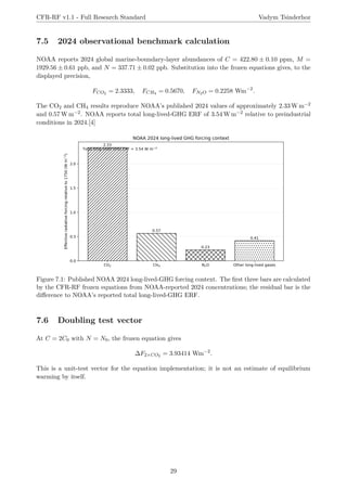
NOAA reports 2024 global marine-boundary-layer abundances of C = 422.80 ± 0.10 ppm, M =
1929.56 ± 0.61 ppb, and N = 337.71 ± 0.02 ppb. Substitution into the frozen equations gives, to the
displayed precision,
FCO2 = 2.3333, FCH4 = 0.5670, FN2O = 0.2258 Wm−2
.
The CO2 and CH4 results reproduce NOAA’s published 2024 values of approximately 2.33 W m−2
and 0.57 W m−2. NOAA reports total long-lived-GHG ERF of 3.54 W m−2 relative to preindustrial
conditions in 2024.[4]
Figure 7.1: Published NOAA 2024 long-lived-GHG forcing context. The first three bars are calculated
by the CFR-RF frozen equations from NOAA-reported 2024 concentrations; the residual bar is the
difference to NOAA’s reported total long-lived-GHG ERF.
7.6 Doubling test vector
At C = 2C0 with N = N0, the frozen equation gives
∆F2×CO2 = 3.93414 Wm−2
.
This is a unit-test vector for the equation implementation; it is not an estimate of equilibrium
warming by itself.
29
31.
Chapter 8
Non-GHG, solar,and volcanic forcing
treatment
8.1 Short-lived anthropogenic forcing
Aerosol-radiation interactions, aerosol-cloud interactions, ozone, land-use albedo, aviation contrails,
black carbon on snow, and related terms have larger structural uncertainty than the direct forcing
from major long-lived greenhouse gases. CFR-RF does not invent simple concentration formulas for
these components. It imports a versioned forcing time series or ensemble from an assessed source
and preserves the source covariance or ensemble structure when available.
8.2 Solar forcing
Solar forcing enters M1, M2, and M8 as a frozen time series derived from total-solar-irradiance
reconstructions or assessed ERF products. A solar-dominant model is not allowed to scale the solar
series by an unconstrained factor chosen after test inspection. If a scaling factor is estimated, its
admissible range and estimation interval must be registered on TRAIN.
8.3 Volcanic forcing
Volcanic forcing is strongly episodic and is commonly represented through stratospheric aerosol
optical depth or an assessed radiative-forcing series. Because major eruptions produce short-lived
cooling, the volcanic component is especially important for checking whether a candidate model can
reproduce transient departures without contaminating the long-term trend estimate.
8.4 Forcing uncertainty
Uncertainty is propagated using published ensemble members when available. If only a mean and
covariance are available, a parametric approximation may be used only if preregistered. The primary
output is not simply a central estimate but the fraction of forcing realizations under which the
decisive attribution gates retain their sign and pass status.
30
32.
Chapter 9
Two-layer energy-balancemodel: con-
tinuous derivation
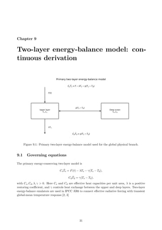
Figure 9.1: Primary two-layer energy-balance model used for the global physical branch.
9.1 Governing equations
The primary energy-conserving two-layer model is
CsṪs = F(t) − λTs − γ(Ts − Td),
CdṪd = γ(Ts − Td),
with Cs, Cd, λ, γ 0. Here Cs and Cd are effective heat capacities per unit area, λ is a positive
restoring coefficient, and γ controls heat exchange between the upper and deep layers. Two-layer
energy-balance emulators are used in IPCC AR6 to connect effective radiative forcing with transient
global-mean temperature response.[2, 3]
31
33.
CFR-RF v1.1 -Full Research Standard Vadym Tsinderhoz
9.2 Energy identity
Summing the two equations eliminates the internal exchange term:
CsṪs + CdṪd = F(t) − λTs = N(t).
This identity is central to the physical branch because it prevents the ocean-exchange parameter
from functioning as a hidden energy source.
9.3 Equilibrium
For constant forcing F∗, setting both derivatives to zero gives Ts = Td. Therefore
T∗
s = T∗
d =
F∗
λ
.
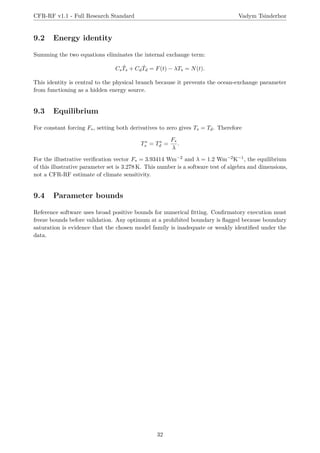
For the illustrative verification vector F∗ = 3.93414 Wm−2 and λ = 1.2 Wm−2K−1, the equilibrium
of this illustrative parameter set is 3.278 K. This number is a software test of algebra and dimensions,
not a CFR-RF estimate of climate sensitivity.
9.4 Parameter bounds
Reference software uses broad positive bounds for numerical fitting. Confirmatory execution must
freeze bounds before validation. Any optimum at a prohibited boundary is flagged because boundary
saturation is evidence that the chosen model family is inadequate or weakly identified under the
data.
32
34.
Chapter 10
State-space form,exact discretization,
and stability
10.1 Continuous state space
Let
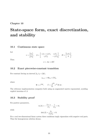
x =
Ts
Td
#
, A =
−(λ + γ)/Cs γ/Cs
γ/Cd −γ/Cd
#
, B =
1/Cs
0
#
.
Then
ẋ = Ax + BF.
10.2 Exact piecewise-constant transition
For constant forcing on interval [tk, tk + ∆t),
xk+1 = Φxk + ΓFk,
where
Φ = eA∆t
, Γ =
Z ∆t
0
eAτ
B dτ.
The reference implementation computes both using an augmented matrix exponential, avoiding
explicit inversion of A.
10.3 Stability proof
For positive parameters,
tr(A) = −
λ + γ
Cs
−
γ
Cd
0,
while
det(A) =
λγ
CsCd
0.
For a real two-dimensional linear system these conditions imply eigenvalues with negative real parts.
Thus the homogeneous solution decays.
33
35.
CFR-RF v1.1 -Full Research Standard Vadym Tsinderhoz
10.4 Numerical verification vector
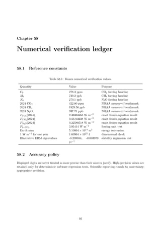
For Cs = 8, Cd = 110, λ = 1.2, γ = 0.7 in consistent yearly units, the eigenvalues are approximately
−0.239884 and −0.003979 yr−1. For ∆t = 1 year,
Φ ≈
0.788834 0.077635
0.005646 0.993913
#
, Γ ≈
0.111275
0.000367
#
.
These values are locked as numerical regression tests for the state-space routine.
34
36.
Chapter 11
Observation model,ocean heat content,
and energy endpoints
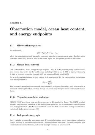
11.1 Observation equation
For endpoint k,
yobs
k,t = hk(xt, θ) + bk,t + ϵk,t,
where b represents structured bias and ϵ represents sampling or measurement noise. An observation
product’s uncertainty model is part of the frozen input, not an optional graphical decoration.
11.2 Ocean heat content
OHC is treated as a direct energy-storage endpoint. NOAA NCEI provides yearly and subannual
heat-content time series for the world ocean, including 0–700 m and 0–2000 m layers, with yearly
0–2000 m products extending through 2025 and subannual fields into 2026.[9]
For a model-predicted change in heat content ∆H over interval ∆t, the corresponding global-mean
heat-flux equivalent is
N̄H =
∆H
AE∆t
.
The framework records the ocean mask, depth interval, reference climatology, and units so that a
mismatch between global Earth-system storage and ocean-only storage is never hidden inside a scale
factor.
11.3 Top-of-atmosphere radiation
CERES EBAF provides a long satellite-era record of TOA radiative fluxes. The EBAF product
applies a constrainment procedure so that its long-term global net flux is consistent with Earth-system
heat storage; therefore CFR-RF does not treat EBAF net flux and the heat-storage constraint as
statistically independent evidence.[10]
11.4 Independence graph
Every endpoint is assigned a provenance node. If two products share source observations, calibration
targets, infilling, or a conservation constraint, that dependence is declared. The multi-endpoint gate
counts independent mechanisms, not merely multiple columns in a spreadsheet.
35
37.
Chapter 12
Internal variabilityand stochastic bench-
marks
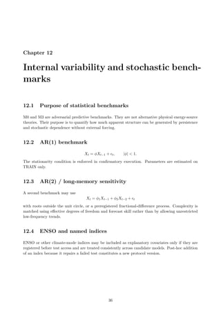
12.1 Purpose of statistical benchmarks
M0 and M3 are adversarial predictive benchmarks. They are not alternative physical energy-source
theories. Their purpose is to quantify how much apparent structure can be generated by persistence
and stochastic dependence without external forcing.
12.2 AR(1) benchmark
Xt = ϕXt−1 + ϵt, |ϕ| 1.
The stationarity condition is enforced in confirmatory execution. Parameters are estimated on
TRAIN only.
12.3 AR(2) / long-memory sensitivity
A second benchmark may use
Xt = ϕ1Xt−1 + ϕ2Xt−2 + ϵt
with roots outside the unit circle, or a preregistered fractional-difference process. Complexity is
matched using effective degrees of freedom and forecast skill rather than by allowing unrestricted
low-frequency trends.
12.4 ENSO and named indices
ENSO or other climate-mode indices may be included as explanatory covariates only if they are
registered before test access and are treated consistently across candidate models. Post-hoc addition
of an index because it repairs a failed test constitutes a new protocol version.
36
Chapter 13
Optimal fingerprinting:formal model
13.1 Regression architecture
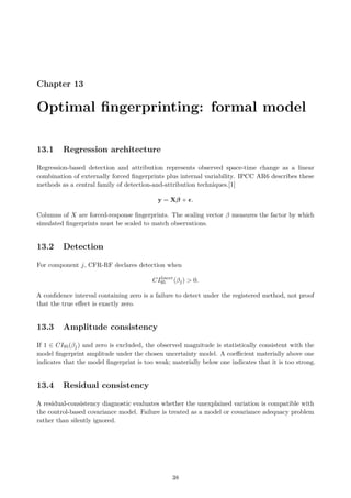
Regression-based detection and attribution represents observed space-time change as a linear
combination of externally forced fingerprints plus internal variability. IPCC AR6 describes these
methods as a central family of detection-and-attribution techniques.[1]
y = Xβ + ϵ.
Columns of X are forced-response fingerprints. The scaling vector β measures the factor by which
simulated fingerprints must be scaled to match observations.
13.2 Detection
For component j, CFR-RF declares detection when
CIlower
95 (βj) 0.
A confidence interval containing zero is a failure to detect under the registered method, not proof
that the true effect is exactly zero.
13.3 Amplitude consistency
If 1 ∈ CI95(βj) and zero is excluded, the observed magnitude is statistically consistent with the
model fingerprint amplitude under the chosen uncertainty model. A coefficient materially above one
indicates that the model fingerprint is too weak; materially below one indicates that it is too strong.
13.4 Residual consistency
A residual-consistency diagnostic evaluates whether the unexplained variation is compatible with
the control-based covariance model. Failure is treated as a model or covariance adequacy problem
rather than silently ignored.
38
40.
Chapter 14
Regularized GLSestimator
14.1 Estimator
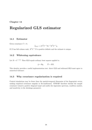
Given covariance C ≻ 0,
β̂GLS = (XT
C−1
X)−1
XT
C−1
y.
If X has full column rank, XT C−1X is positive definite and the estimate is unique.
14.2 Whitening equivalence
Let R = C−1/2. Then GLS equals ordinary least squares applied to
ỹ = Ry, X̃ = RX.
This identity provides a useful implementation test: direct GLS and whitened OLS must agree to
numerical tolerance.
14.3 Why covariance regularization is required
Control simulations may be fewer than the spatial-temporal dimension of the fingerprint vector,
making empirical covariance singular or ill-conditioned. CFR-RF therefore shrinks the sample
covariance toward a positive diagonal target and audits the eigenvalue spectrum, condition number,
and sensitivity to the shrinkage parameter.
39
41.
Chapter 15
Errors-in-variables andcovariance-whitened
TLS sensitivity
15.1 Motivation
Fingerprint columns are themselves estimated from finite climate-model ensembles and therefore
contain noise. Ordinary GLS treats regressors as fixed. Errors-in-variables methods address this
asymmetry.
15.2 Whitened TLS reference
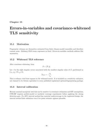
After covariance whitening, form
Z = [X̃ ỹ].
Let v be the right singular vector associated with the smallest singular value of Z, partitioned as
(vX, vy). If vy ̸= 0,
β̂TLS = −
vX
vy
.
This is ordinary total least squares in the whitened metric. It is included as a sensitivity estimator,
not claimed to be bitwise equivalent to every published regularized optimal-fingerprinting package.
15.3 Interval calibration
Because nominal asymptotic intervals can be sensitive to covariance estimation and EIV assumptions,
CFR-RF requires perfect-model or synthetic coverage experiments before applying the strong
detection gate. If a 95% interval method has material undercoverage in the registered design, the
interval method fails validation even if its point estimate appears plausible.
40
42.
Chapter 16
Covariance estimationand regulariza-
tion
16.1 Sample covariance
For centered control vectors zi,
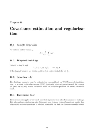
S =
1
n − 1
n
X
i=1
zizT
i .
16.2 Diagonal shrinkage
Define T = diag(S) and
Cρ = (1 − ρ)S + ρT, 0 ρ ≤ 1.
If the diagonal variances are strictly positive, Cρ is positive definite for ρ 0.
16.3 Selection rule
The shrinkage parameter may be estimated or cross-validated on TRAIN/control simulations
only. It is frozen before observational TEST. Sensitivity values are pre-registered, for example
ρ ∈ {0.05, 0.1, 0.2, 0.4}, so that one cannot select the value that produces the desired attribution
result.
16.4 Eigenvalue floor
The reference code applies a very small numerical eigenvalue floor only after documented shrinkage.
This safeguard prevents floating-point failure and must be many orders of magnitude smaller than
substantively relevant eigenvalues. If inference depends on the floor, the covariance model is invalid.
41
43.
Chapter 17
Serial correlation,blocked resampling,
and interval construction
17.1 Why iid bootstrap is unsuitable
Annual and monthly climate time series exhibit temporal dependence. Sampling individual time
points independently destroys this structure and can understate uncertainty. The primary time-series
skill comparison therefore uses moving-block or stationary bootstrap variants.
17.2 Moving-block bootstrap
For block length L, resample contiguous blocks with replacement until the test-length series is
reconstructed. Compared models use identical resampled indices so that skill differences are paired.
17.3 Frozen block lengths
For monthly analyses the primary block length is 60 months, with sensitivity at 24 and 120 months.
For annual analyses, a separate preregistered block length is selected using TRAIN autocorrelation
diagnostics. A conclusion that changes sign across all reasonable frozen block choices is reported as
Unstable.
17.4 Confidence intervals
For relative skill S(b) from bootstrap replicate b, the primary interval is the percentile interval unless
a calibrated alternative is registered. The gate requires the lower 95% bound to exceed zero in
addition to the practical 5% skill threshold.
42
44.
Chapter 18
Forcing uncertaintypropagation
18.1 Ensemble propagation
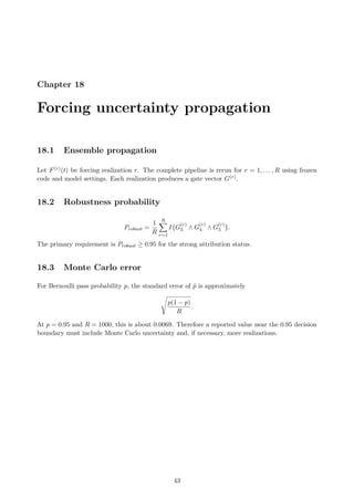
Let F(r)(t) be forcing realization r. The complete pipeline is rerun for r = 1, . . . , R using frozen
code and model settings. Each realization produces a gate vector G(r).
18.2 Robustness probability
Probust =
1
R
R
X
r=1
I{G
(r)
3 ∧ G
(r)
4 ∧ G
(r)
5 }.
The primary requirement is Probust ≥ 0.95 for the strong attribution status.
18.3 Monte Carlo error
For Bernoulli pass probability p, the standard error of p̂ is approximately
s
p(1 − p)
R
.
At p = 0.95 and R = 1000, this is about 0.0069. Therefore a reported value near the 0.95 decision
boundary must include Monte Carlo uncertainty and, if necessary, more realizations.
43
45.
Chapter 19
Predictive metricsand practical signifi-
cance
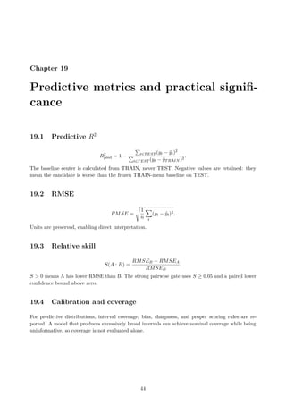
19.1 Predictive R2
R2
pred = 1 −
P
t∈TEST (yt − ŷt)2
P
t∈TEST (yt − ȳTRAIN )2
.
The baseline center is calculated from TRAIN, never TEST. Negative values are retained: they
mean the candidate is worse than the frozen TRAIN-mean baseline on TEST.
19.2 RMSE
RMSE =
s
1
n
X
t
(yt − ŷt)2.
Units are preserved, enabling direct interpretation.
19.3 Relative skill
S(A : B) =
RMSEB − RMSEA
RMSEB
.
S 0 means A has lower RMSE than B. The strong pairwise gate uses S ≥ 0.05 and a paired lower
confidence bound above zero.
19.4 Calibration and coverage
For predictive distributions, interval coverage, bias, sharpness, and proper scoring rules are re-
ported. A model that produces excessively broad intervals can achieve nominal coverage while being
uninformative, so coverage is not evaluated alone.
44
46.
Chapter 20
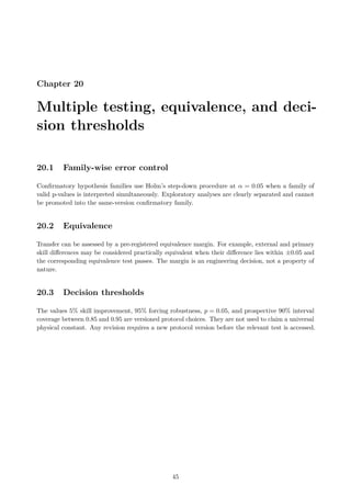
Multiple testing,equivalence, and deci-
sion thresholds
20.1 Family-wise error control
Confirmatory hypothesis families use Holm’s step-down procedure at α = 0.05 when a family of
valid p-values is interpreted simultaneously. Exploratory analyses are clearly separated and cannot
be promoted into the same-version confirmatory family.
20.2 Equivalence
Transfer can be assessed by a pre-registered equivalence margin. For example, external and primary
skill differences may be considered practically equivalent when their difference lies within ±0.05 and
the corresponding equivalence test passes. The margin is an engineering decision, not a property of
nature.
20.3 Decision thresholds
The values 5% skill improvement, 95% forcing robustness, p = 0.05, and prospective 90% interval
coverage between 0.85 and 0.95 are versioned protocol choices. They are not used to claim a universal
physical constant. Any revision requires a new protocol version before the relevant test is accessed.
45
47.
Chapter 21
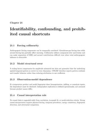
Identifiability, confounding,and prohib-
ited causal shortcuts
21.1 Forcing collinearity
Anthropogenic forcing components can be temporally correlated. Greenhouse-gas forcing rises while
aerosol forcing has partially offset warming. Collinearity inflates component-wise uncertainty and
can make separation of GHG and aerosol contributions difficult even when total anthropogenic
influence is detectable.
21.2 Model structural error
A scaling factor compensates for amplitude mismatch but does not guarantee that the underlying
spatial-temporal pattern is correct in every dimension. CFR-RF therefore reports pattern residuals
and transfer behavior rather than reducing attribution to one coefficient.
21.3 Observation-model dependence
If a temperature product and model fingerprint share homogenization, infilling, or reanalysis inputs,
the dependence must be disclosed. Independent replication is defined operationally, not assumed
because product names differ.
21.4 Causal interpretation rule
No causal claim is upgraded solely from correlation, in-sample fit, or model-selection criteria. Strong
causal interpretation requires physical forcing, temporal precedence, energy consistency, fingerprint
detection, and adversarial comparison.
46
Chapter 22
Overview ofM0–M8
Figure 22.1: Frozen candidate-model channels. “Internal stochastic” is included as a residual/bench-
mark process where applicable; it is not an external forcing source.
22.1 Common rules
All models use the same temporal splits, observation transformations, missing-data masks, and
primary metrics. A model may not receive additional post-hoc basis functions, lags, or forcing
rescaling unavailable to its competitors. Physical models must pass positivity and energy-accounting
checks. Statistical benchmarks may win forecast skill but cannot by that fact alone establish a
physical cause.
22.2 Complexity reporting
Each model report includes the number of fitted continuous parameters, discrete hyperparameters,
effective degrees of freedom where available, and all constraints. Head-to-head interpretation is
48
50.
CFR-RF v1.1 -Full Research Standard Vadym Tsinderhoz
invalid if one model has hidden outcome-informed flexibility.
22.3 Common model-output contract
Every M0–M8 execution emits fitted parameters, physical-bound status where applicable, TEST
RMSE, predictive R2, paired skill differences, uncertainty intervals, residual diagnostics, input
hashes, and an immutable model-configuration hash. Physical models additionally emit implied net
imbalance, heat-storage consistency, forcing-channel contributions, and any boundary-saturation
diagnostics. This common contract is specified once here and applies to every registered model.
49
51.
Chapter 23
M0 -NULL-AR1
23.1 Mechanism
Stationary internal benchmark.
23.2 Formal specification
No external forcing. Tt = µ + ϕ(Tt−1 − µ) + ϵt, |ϕ| 1.
23.3 Scientific purpose
Provides a persistence benchmark. It can pass temperature forecast metrics but cannot pass the
external-energy attribution gate.
23.4 Mandatory failure conditions
Non-stationarity, hidden trend terms, or test-selected breaks invalidate the registered M0.
50
52.
Chapter 24
M1 -NAT
24.1 Mechanism
Natural-forcing physical model.
24.2 Formal specification
F(t) = Fsolar(t) + Fvolc(t) drives the same frozen EBM used by other physical models.
24.3 Scientific purpose
Tests whether assessed natural forcing plus internal residual variability can account for held-out
temperature and energy endpoints.
24.4 Mandatory failure conditions
If natural-only skill is materially below ALL, energy storage is unexplained, or parameters leave
physical bounds, M1 fails the strong natural explanation.
51

53.
Chapter 25
M2 -SOLAR
25.1 Mechanism
Solar-dominant physical model.
25.2 Formal specification
F(t) = Fsolar(t) with a pre-registered scaling/uncertainty treatment only.
25.3 Scientific purpose
Directly tests a common alternative claim that solar variability dominates modern warming.
25.4 Mandatory failure conditions
It must predict long-term temperature, OHC/EEI, and fingerprints. Post-hoc amplification of solar
forcing is prohibited.
52
54.
Chapter 26
M3 -INTERNAL
26.1 Mechanism
Higher-order internal stochastic benchmark.
26.2 Formal specification
AR(2), state-space stochastic, or frozen long-memory process without external energy input.
26.3 Scientific purpose
Stress-tests whether low-frequency persistence alone can predict the held-out record.
26.4 Mandatory failure conditions
A hidden deterministic trend or nonzero-mean external energy term changes the model class and
invalidates M3.
53
55.
Chapter 27
M4 -OBS-BIAS+NAT
27.1 Mechanism
Bounded observational-bias alternative.
27.2 Formal specification
Tobs
t = Ttrue
t + bt + ϵt, with Ttrue driven by NAT and bt constrained by the frozen observational
uncertainty model.
27.3 Scientific purpose
Tests whether a substantial portion of apparent warming can plausibly arise from measurement/pro-
cessing bias.
27.4 Mandatory failure conditions
If the required bias exceeds the product uncertainty envelope or fails independent OHC/radiation
evidence, M4 fails.
54
56.
Chapter 28
M5 -ANT-NONGHG
28.1 Mechanism
Anthropogenic non-ghg model.
28.2 Formal specification
F = Faer + FO3 + FLU + Fcontrail + Fother, excluding well-mixed GHG.
28.3 Scientific purpose
Tests whether non-GHG anthropogenic forcing can explain the response without a dominant GHG
contribution.
28.4 Mandatory failure conditions
Poor out-of-sample skill or inability to reproduce positive long-term forcing-response behavior rejects
M5.
55
57.
Chapter 29
M6 -GHG
29.1 Mechanism
Well-mixed greenhouse-gas model.
29.2 Formal specification
F = FCO2 + FCH4 + FN2O + Fhalo.
29.3 Scientific purpose
Tests the predictive information carried by well-mixed GHG forcing without short-lived anthropogenic
or natural terms.
29.4 Mandatory failure conditions
Failure to transfer or explain energy endpoints limits the inference even if temperature fit is strong.
56
58.
Chapter 30
M7 -ANT
30.1 Mechanism
All-anthropogenic model.
30.2 Formal specification
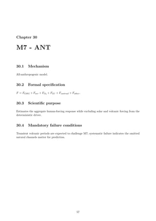
F = FGHG + Faer + FO3 + FLU + Fcontrail + Fother.
30.3 Scientific purpose
Estimates the aggregate human-forcing response while excluding solar and volcanic forcing from the
deterministic driver.
30.4 Mandatory failure conditions
Transient volcanic periods are expected to challenge M7; systematic failure indicates the omitted
natural channels matter for prediction.
57
59.
Chapter 31
M8 -ALL
31.1 Mechanism
Full physical model.
31.2 Formal specification
F = FANT + Fsolar + Fvolc with frozen forcing uncertainty and the primary EBM.
31.3 Scientific purpose
Primary strong competitor: tests the joint anthropogenic-plus-natural physical explanation.
31.4 Mandatory failure conditions
Strong status requires G0–G8 and, for the highest prospective status, G9. Good in-sample fit alone
is insufficient.
58
60.
Chapter 32
Neutral black-boxpredictive benchmark
32.1 Purpose
A neutral machine-learning or statistical benchmark may be included to test whether the physical
architecture provides predictive information beyond a generic model of comparable complexity. The
black-box benchmark is not assigned a causal interpretation.
32.2 Allowed forms
Candidates include regularized autoregression, Gaussian-process regression, or state-space mod-
els with frozen kernels and hyperparameter ranges. Hyperparameters are selected only within
TRAIN/VALIDATION. The benchmark must receive only variables that would have been available
at prediction time.
32.3 Fairness condition
If the black-box model receives future forcing, revised observations, or target-derived features
unavailable to a physical competitor, the comparison is invalid. Conversely, physical models cannot
be given test-tuned forcing scalings unavailable to the black-box benchmark.
59
Chapter 33
Data inventoryand source hierarchy
33.1 Primary source families
The baseline execution uses versioned, authoritative sources for global surface temperature, greenhouse-
gas abundance and forcing, assessed aggregate forcing, ocean heat content, satellite radiation, and
climate-model fingerprints. The framework never treats a web page name as a sufficient version
identifier. A local byte snapshot and cryptographic hash are required.
Table 33.1: Baseline data-source registry.
Source Baseline version Coverage CFR-RF role
IGCC 2025 v2026.06.15 forcing 1750–
2025; GMST
1850–2025; EEI
1971–2025
aggregate assessed forcing,
attribution-context data, energy
indicators
HadCRUT5 5.1.0.0 1850–present primary global surface-temperature
product and uncertainty ensemble
GISTEMP v4 snapshot at lock 1880–present external transfer temperature prod-
uct
NOAA AGGI 2024 release, page
updated 2025
1750 baseline;
observations
through 2024
exact long-lived-GHG ERF equations
and measured concentrations
NOAA NCEI OHC snapshot at lock yearly 1955–
2025; subannual
updates into
2026
ocean heat-storage endpoint
CERES EBAF Ed4.2/4.2.1, DQS
V7
Mar 2000–
present
satellite radiation sensitivity branch
and spatial/temporal radiation diag-
nostics
CMIP6/DAMIP explicit ESGF track-
ing IDs
model-
dependent
forced fingerprints and control vari-
ability
The IGCC 2025 release on Zenodo explicitly contains ERF through 2025, GMST through 2025,
historical attribution through 2025, and EEI through 2025; the release is version v2026.06.15 and
publishes an upstream archive MD5. CFR-RF computes its own SHA-256 after byte acquisition.[6]
61
63.
Chapter 34
HadCRUT5 temperatureproduct
34.1 Version
The baseline is HadCRUT.5.1.0.0. Met Office release notes identify it as the current HadCRUT5
version and describe updates to CRUTEM, HadSST, and sea-ice inputs relative to 5.0.2.0.[7]
34.2 Use in CFR-RF
The framework uses the annual global series for primary scalar temperature evaluation and can use
the gridded ensemble for fingerprint and uncertainty analyses. The 1850–1900 mean is a reporting
reference; model fitting and prediction use anomalies aligned according to the frozen canonical
schema.
34.3 Uncertainty handling
If an ensemble of observational realizations is provided, uncertainty is propagated across the ensemble
rather than replacing it with a single standard-error band. Any change in the upstream product
version requires a new local snapshot and hash; it cannot silently replace the locked input.
62
64.
Chapter 35
NASA GISTEMPv4 transfer product
35.1 Versioning
NASA GISTEMP v4 is updated around the middle of each month and uses GHCN v4 land
observations with ERSST v5 ocean data. Because late reports and corrections can revise earlier
months, the exact CFR-RF input is the local file snapshot and retrieval timestamp, not merely the
label “GISTEMP v4.”[8]
35.2 Transfer role
GISTEMP is used as an external observational processing branch for the transfer gate. Its different
spatial processing and reference conventions require a frozen anomaly-alignment transformation
before comparison. The transfer test asks whether the sign and practical magnitude of model
advantage survive a different observation product, not whether the raw numerical anomaly values
are identical.
63
65.
Chapter 36
Indicators ofGlobal Climate Change
2025 baseline
36.1 Published context
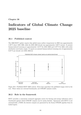
The 2026 IGCC update reports that global mean surface temperature in 2025 was approximately
1.39 °C above 1850–1900, while the 2016–2025 decade was approximately 1.26 °C warmer. It assesses
human-induced warming at approximately 1.24 °C for 2016–2025 and 1.37 °C for 2025, with wider
attribution uncertainty ranges. It reports an assessed human-induced warming rate of approximately
0.27 °C per decade over 2016–2025.[5]
Figure 36.1: Published IGCC 2025 context. Error bars reproduce the published ranges cited in the
text. These values are external benchmarks, not CFR-RF analysis results.
36.2 Role in the framework
IGCC provides a convenient versioned aggregate source for forcing and energy indicators and a
benchmark against which CFR-RF outputs can be sanity-checked. Agreement with IGCC is not
automatically a PASS; the decisive outputs are generated by the frozen CFR-RF pipeline from its
locked inputs.
64
66.
Chapter 37
NOAA greenhouse-gasobservational base-
line
37.1 Measured abundances
NOAA GML reports 2024 global marine-boundary-layer averages of 422.80 ppm CO2, 1929.56 ppb
CH4, and 337.71 ppb N2O, each with small measurement uncertainty. It reports total long-lived-GHG
ERF of approximately 3.54 W m−2 relative to preindustrial conditions.[4]
37.2 Use
These values serve as direct numerical verification of the forcing code and as an independent
observational input for the concentration-derived long-lived-GHG branch. The broader anthropogenic
forcing vector still requires aerosol, ozone, land-use, contrail, and other terms from an assessed
forcing dataset.
65
67.
Chapter 38
NOAA oceanheat content endpoint
38.1 Coverage
NOAA NCEI provides global and basin OHC time series for 0–700 m and 0–2000 m layers. The
current public pages describe yearly series through 2025 and subannual values into 2026.[9]
38.2 Canonical transformation
The canonical annual table stores OHC in joules and preserves the source standard error. Source
files expressed in 1022 J are converted by an explicit multiplier and the conversion is unit-tested. No
missing year is replaced by zero.
38.3 Role in G2 and G6
The energy accumulation gate checks the sign and uncertainty of heat-content change and its
consistency with model-implied net energy imbalance. The multi-endpoint fingerprint gate uses
OHC as a mechanism-distinct line of evidence from surface temperature.
66
68.
Chapter 39
CERES EBAFradiation branch and
dependence policy
39.1 Version
CERES EBAF Edition 4.2/4.2.1 Data Quality Summary Version 7 was released 1 July 2026. It
documents satellite transitions and the EBAF constrainment algorithm.[10]
39.2 Constrainment dependence
CERES notes that raw global net TOA imbalance exceeds expected Earth-system heat storage
and that EBAF adjusts SW and LW TOA fluxes within uncertainty to remove this inconsistency.
Therefore the balanced net-flux mean is not independent of heat-storage knowledge. CFR-RF uses
CERES for radiation variability, spatial fingerprints, and sensitivity analyses while preventing false
multiplication of independent evidence.
39.3 Satellite transitions
The data-quality document records Terra-only, Terra+Aqua, and NOAA-20-only periods and
climatological adjustments across transitions. CFR-RF marks these change points in the provenance
metadata so that trend diagnostics can test sensitivity to platform transitions.
67
69.
Chapter 40
CMIP6/DAMIP fingerprintsand con-
trol variability
40.1 Required experiment classes
Full optimal fingerprinting requires climate-model simulations that isolate forcing classes, for example
historical all-forcing, greenhouse-gas-only, natural-only, or other-anthropogenic experiments, along
with long preindustrial control simulations for internal variability.
40.2 File-level lock
Every netCDF input must be identified by institution, source model, experiment, member/variant
label, grid, version or ESGF tracking identifier, variable, temporal range, and SHA-256. Changing
the model ensemble after observation TEST inspection is prohibited.
40.3 Fingerprint construction
The spatial-temporal fingerprint operator, regridding, masking, area weighting, temporal averaging,
and dimensional reduction are all frozen before the confirmatory observation vector is evaluated. If
a model fingerprint has been selected because it resembles observations, the resulting attribution
must be downgraded or invalidated due to circular selection.
68
70.
Chapter 41
Canonical annualschema and unit dis-
cipline
41.1 Core columns
The canonical annual table contains at least: year, temperature anomaly and uncertainty per product,
CO2/CH4/N2O abundance, component ERF terms, total anthropogenic and natural ERF, OHC
and uncertainty, radiation diagnostics, data-availability flags, and source-version identifiers.
41.2 Units
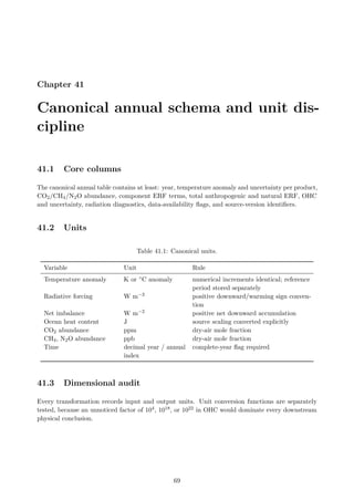
Table 41.1: Canonical units.
Variable Unit Rule
Temperature anomaly K or ◦C anomaly numerical increments identical; reference
period stored separately
Radiative forcing W m−2 positive downward/warming sign conven-
tion
Net imbalance W m−2 positive net downward accumulation
Ocean heat content J source scaling converted explicitly
CO2 abundance ppm dry-air mole fraction
CH4, N2O abundance ppb dry-air mole fraction
Time decimal year / annual
index
complete-year flag required
41.3 Dimensional audit
Every transformation records input and output units. Unit conversion functions are separately
tested, because an unnoticed factor of 104, 1018, or 1022 in OHC would dominate every downstream
physical conclusion.
69
71.
Chapter 42
Byte locking,SHA-256, and provenance
manifest
42.1 Data lock object
For each input file, the manifest records source URL or DOI, retrieval timestamp, upstream version,
local path, byte size, SHA-256 digest, and optional upstream checksum. The local SHA-256 is
authoritative for reproducibility.
42.2 Mutable products
Products such as GISTEMP and ongoing NOAA/CERES time series are routinely revised. Therefore
“same dataset name” does not imply “same data.” Revisions after the lock are new inputs and belong
to a new execution or protocol version.
42.3 Manifest verification
Before any test run, the pipeline recomputes every digest and refuses confirmatory execution if any
file differs. The code, configuration, model registry, and environment lock are hashed as well.
70
72.
Chapter 43
Temporal firewall:1750–2031
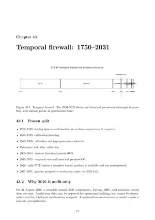
Figure 43.1: Temporal firewall. The 2000–2025 blocks are historical pseudo-out-of-sample because
they were already public at specification time.
43.1 Frozen split
• 1750–1849: forcing spin-up and baseline; no surface-temperature fit required.
• 1850–1979: calibration/training.
• 1980–1999: validation and hyperparameter selection.
• Parameter lock after validation.
• 2000–2014: internal historical pseudo-OOS.
• 2015–2025: temporal external historical pseudo-OOS.
• 2026: audit-YTD unless a complete annual product is available and was preregistered.
• 2027–2031: genuine prospective evaluation under the 2026 lock.
43.2 Why 2026 is audit-only
On 24 August 2026, a complete annual 2026 temperature, forcing, OHC, and radiation record
does not exist. Partial-year data may be inspected for operational auditing, but cannot be silently
substituted for a full-year confirmatory endpoint. A seasonal-to-annual estimator would require a
separate preregistration.
71
73.
CFR-RF v1.1 -Full Research Standard Vadym Tsinderhoz
Figure 43.2: Evidence hierarchy. Genuinely post-lock observations have the strongest protection
against retrospective tuning.
72
Chapter 44
G0–G9 overview
Figure44.1: Mandatory decision chain. G0 integrity dominates all higher scientific statuses.
A gate is a versioned decision rule. Passing a later gate cannot repair failure of an earlier mandatory
gate. Some intermediate scientific statements use a subset of gates, while the strongest attribution
statement requires the conjunction specified below.
44.1 Common gate-audit record
For every G0–G9 decision, the machine report records the raw statistic, interval, threshold, Boolean
result, input manifest ID, execution timestamp, software commit/hash, and sensitivity status.
Human-readable interpretation never replaces the raw decision record. Gate-specific chapters
therefore state only their unique PASS, FAIL/INVALID, and scientific-meaning conditions.
74
76.
Chapter 45
G0 -Integrity
45.1 PASS criterion
All locked input, code, model, environment, and configuration hashes match; no outcome-bearing
access occurred before lock; zero documented leakage.
45.2 FAIL/INVALID criterion
Any hash mismatch, test-informed model modification, unlogged data substitution, or broken access
firewall yields INVALID.
45.3 Scientific meaning
Protects every downstream inference from silent version drift or data leakage.
75
77.
Chapter 46
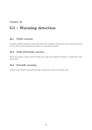
G1 -Warming detection
46.1 PASS criterion
A positive global-temperature trend with lower 95% confidence bound above zero, reproduced across
at least three frozen temperature products or processing branches.
46.2 FAIL/INVALID criterion
Trend not positive, lower bound includes zero under the registered method, or replication count
below three.
46.3 Scientific meaning
Answers only whether sustained warming is observed; it does not identify cause.
76
78.
Chapter 47
G2 -Energy accumulation
47.1 PASS criterion
OHC/energy-storage trend has lower confidence bound above zero and is sign-consistent with
model-implied net imbalance over the registered interval.
47.2 FAIL/INVALID criterion
No robust energy accumulation, sign inconsistency, or unresolved unit/reference mismatch.
47.3 Scientific meaning
Separates surface redistribution from persistent whole-system energy gain.
77
79.
Chapter 48
G3 -Anthropogenic detection
48.1 PASS criterion
Lower 95% bound of anthropogenic fingerprint scaling factor exceeds zero and residual-consistency
diagnostic passes.
48.2 FAIL/INVALID criterion
Anthropogenic coefficient is not detected or covariance/residual model fails calibration.
48.3 Scientific meaning
Establishes detection under the registered fingerprinting design, not exclusive causation.
78
80.
Chapter 49
G4 -ALL versus NAT
49.1 PASS criterion
M8 improves held-out skill over M1 by at least 5%, paired lower CI 0, with same-direction advantage
on an energy-relevant endpoint.
49.2 FAIL/INVALID criterion
Skill gain below 5%, interval includes zero, or energy endpoint points in the opposite direction.
49.3 Scientific meaning
Direct adversarial test of full forcing against natural-only forcing.
79
81.
Chapter 50
G5 -GHG ablation
50.1 PASS criterion
Removing GHG forcing from the full model worsens held-out skill by at least 5% with lower CI 0.
50.2 FAIL/INVALID criterion
Ablation has no robust loss or improves performance.
50.3 Scientific meaning
Tests incremental predictive information of GHG conditional on the registered architecture.
80
82.
Chapter 51
G6 -Multi-endpoint fingerprints
51.1 PASS criterion
Surface temperature, OHC/energy, and radiation/energy fingerprint requirements pass, plus at least
one preregistered vertical or spatial fingerprint.
51.2 FAIL/INVALID criterion
Temperature alone passes while mandatory non-temperature fingerprints fail.
51.3 Scientific meaning
Prevents a one-series explanation from receiving the strongest causal status.
81
83.
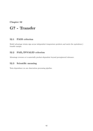
Chapter 52
G7 -Transfer
52.1 PASS criterion
Model advantage retains sign across independent temperature products and meets the equivalence/-
transfer margin.
52.2 FAIL/INVALID criterion
Advantage reverses or is materially product-dependent beyond preregistered tolerance.
52.3 Scientific meaning
Tests dependence on one observation processing pipeline.
82
84.
Chapter 53
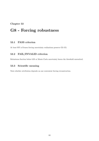
G8 -Forcing robustness
53.1 PASS criterion
At least 95% of frozen forcing uncertainty realizations preserve G3–G5.
53.2 FAIL/INVALID criterion
Robustness fraction below 0.95 or Monte Carlo uncertainty leaves the threshold unresolved.
53.3 Scientific meaning
Tests whether attribution depends on one convenient forcing reconstruction.
83
85.
Chapter 54
G9 -Prospective prediction
54.1 PASS criterion
Post-lock 2027–2031 observations meet registered calibration, coverage, bias, and skill criteria without
model changes.
54.2 FAIL/INVALID criterion
Systematic predictive bias, gross under/overcoverage, or any post-lock retuning in the same version.
54.3 Scientific meaning
Provides genuinely prospective evidence unavailable to the architect at lock time.
84
86.
Chapter 55
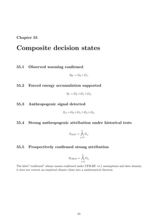
Composite decisionstates
55.1 Observed warming confirmed
SW = G0 ∧ G1.
55.2 Forced energy accumulation supported
SF = G0 ∧ G1 ∧ G2.
55.3 Anthropogenic signal detected
SA = G0 ∧ G1 ∧ G2 ∧ G3.
55.4 Strong anthropogenic attribution under historical tests
SANT =
8
^
j=0
Gj.
55.5 Prospectively confirmed strong attribution
SPROS =
9
^
j=0
Gj.
The label “confirmed” always means confirmed under CFR-RF v1.1 assumptions and data domain;
it does not convert an empirical climate claim into a mathematical theorem.
85
87.
Chapter 56
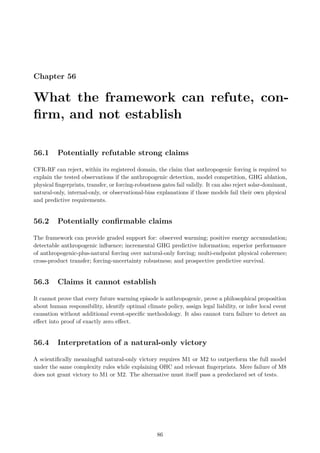
What theframework can refute, con-
firm, and not establish
56.1 Potentially refutable strong claims
CFR-RF can reject, within its registered domain, the claim that anthropogenic forcing is required to
explain the tested observations if the anthropogenic detection, model competition, GHG ablation,
physical fingerprints, transfer, or forcing-robustness gates fail validly. It can also reject solar-dominant,
natural-only, internal-only, or observational-bias explanations if those models fail their own physical
and predictive requirements.
56.2 Potentially confirmable claims
The framework can provide graded support for: observed warming; positive energy accumulation;
detectable anthropogenic influence; incremental GHG predictive information; superior performance
of anthropogenic-plus-natural forcing over natural-only forcing; multi-endpoint physical coherence;
cross-product transfer; forcing-uncertainty robustness; and prospective predictive survival.
56.3 Claims it cannot establish
It cannot prove that every future warming episode is anthropogenic, prove a philosophical proposition
about human responsibility, identify optimal climate policy, assign legal liability, or infer local event
causation without additional event-specific methodology. It also cannot turn failure to detect an
effect into proof of exactly zero effect.
56.4 Interpretation of a natural-only victory
A scientifically meaningful natural-only victory requires M1 or M2 to outperform the full model
under the same complexity rules while explaining OHC and relevant fingerprints. Mere failure of M8
does not grant victory to M1 or M2. The alternative must itself pass a predeclared set of tests.
86
Chapter 57
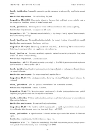
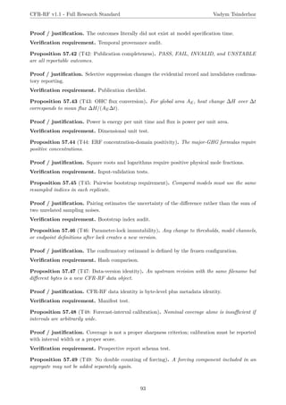
Formal propositionsT1–T50
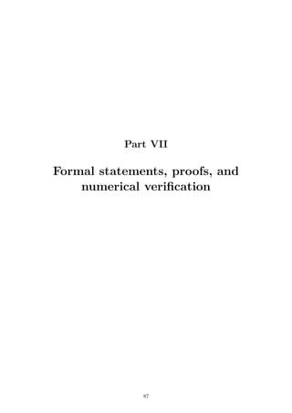
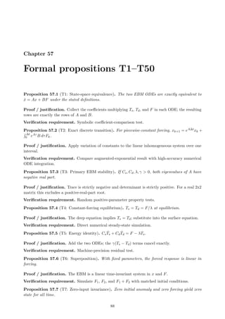
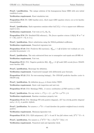
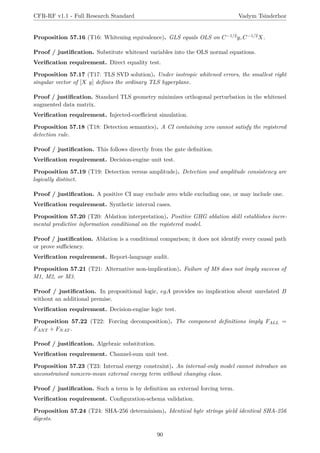
Proposition 57.1 (T1: State-space equivalence). The two EBM ODEs are exactly equivalent to
ẋ = Ax + BF under the stated definitions.
Proof / justification. Collect the coefficients multiplying Ts, Td, and F in each ODE; the resulting
rows are exactly the rows of A and B.
Verification requirement. Symbolic coefficient-comparison test.
Proposition 57.2 (T2: Exact discrete transition). For piecewise-constant forcing, xk+1 = eA∆txk +
R ∆t
0 eAτ B dτFk.
Proof / justification. Apply variation of constants to the linear inhomogeneous system over one
interval.
Verification requirement. Compare augmented-exponential result with high-accuracy numerical
ODE integration.
Proposition 57.3 (T3: Primary EBM stability). If Cs, Cd, λ, γ 0, both eigenvalues of A have
negative real part.
Proof / justification. Trace is strictly negative and determinant is strictly positive. For a real 2x2
matrix this excludes a positive-real-part root.
Verification requirement. Random positive-parameter property tests.
Proposition 57.4 (T4: Constant-forcing equilibrium). Ts = Td = F/λ at equilibrium.
Proof / justification. The deep equation implies Ts = Td; substitute into the surface equation.
Verification requirement. Direct numerical steady-state simulation.
Proposition 57.5 (T5: Energy identity). CsṪs + CdṪd = F − λTs.
Proof / justification. Add the two ODEs; the γ(Ts − Td) terms cancel exactly.
Verification requirement. Machine-precision residual test.
Proposition 57.6 (T6: Superposition). With fixed parameters, the forced response is linear in
forcing.
Proof / justification. The EBM is a linear time-invariant system in x and F.
Verification requirement. Simulate F1, F2, and F1 + F2 with matched initial conditions.
Proposition 57.7 (T7: Zero-input invariance). Zero initial anomaly and zero forcing yield zero
state for all time.
88
90.
CFR-RF v1.1 -Full Research Standard Vadym Tsinderhoz
Proof / justification. The unique solution of the homogeneous linear ODE with zero initial
condition is zero.
Verification requirement. Exact simulation test.
Proposition 57.8 (T8: GHG baseline zero). Each major-GHG equation returns zero at its baseline
concentrations.
Proof / justification. Each expression contains either ln(C/C0) = 0 or a square-root difference
equal to zero.
Verification requirement. Unit tests at C0, M0, N0.
Proposition 57.9 (T9: Doubled-CO2 reference). The frozen equation returns 3.93414 W m−2 at
C = 2C0 and N = N0 to 1e-4.
Proof / justification. Direct substitution using the NOAA-published coefficients.
Verification requirement. Numerical regression test.
Proposition 57.10 (T10: Predictive R2 exactness). R2
pred = 1 iff all finite test residuals are zero,
provided denominator 0.
Proof / justification. The ratio subtracted from one is nonnegative and equals zero iff SSE=0.
Verification requirement. Unit test.
Proposition 57.11 (T11: Negative predictive R2). R2
pred 0 iff model SSE exceeds frozen TRAIN-
mean baseline SSE.
Proof / justification. Rearrange the definition.
Verification requirement. Constructed example with deliberately poor forecasts.
Proposition 57.12 (T12: No test-centering leakage). The CFR-RF predictive baseline center is
TRAIN-only.
Proof / justification. By definition ȳTRAIN is frozen before TEST.
Verification requirement. Static code inspection and unit test.
Proposition 57.13 (T13: Shrinkage PSD). A convex combination of PSD matrices is PSD.
Proof / justification. For any vector v, vT Cρv = (1 − ρ)vT Sv + ρvT Tv ≥ 0.
Verification requirement. Random covariance property test.
Proposition 57.14 (T14: Shrinkage PD with positive diagonal). If T has strictly positive diagonal
and ρ 0, Cρ is positive definite.
Proof / justification. For nonzero v, vT Tv 0 and therefore the positive weighted term is strictly
positive.
Verification requirement. Minimum-eigenvalue test.
Proposition 57.15 (T15: GLS uniqueness). If C ≻ 0 and X has full column rank, XT C−1X ≻ 0.
Proof / justification. For nonzero a, aT XT C−1Xa = (Xa)T C−1(Xa) 0.
Verification requirement. Numerical rank and eigenvalue check.
89
91.
CFR-RF v1.1 -Full Research Standard Vadym Tsinderhoz
Proposition 57.16 (T16: Whitening equivalence). GLS equals OLS on C−1/2y, C−1/2X.
Proof / justification. Substitute whitened variables into the OLS normal equations.
Verification requirement. Direct equality test.
Proposition 57.17 (T17: TLS SVD solution). Under isotropic whitened errors, the smallest right
singular vector of [X y] defines the ordinary TLS hyperplane.
Proof / justification. Standard TLS geometry minimizes orthogonal perturbation in the whitened
augmented data matrix.
Verification requirement. Injected-coefficient simulation.
Proposition 57.18 (T18: Detection semantics). A CI containing zero cannot satisfy the registered
detection rule.
Proof / justification. This follows directly from the gate definition.
Verification requirement. Decision-engine unit test.
Proposition 57.19 (T19: Detection versus amplitude). Detection and amplitude consistency are
logically distinct.
Proof / justification. A positive CI may exclude zero while excluding one, or may include one.
Verification requirement. Synthetic interval cases.
Proposition 57.20 (T20: Ablation interpretation). Positive GHG ablation skill establishes incre-
mental predictive information conditional on the registered model.
Proof / justification. Ablation is a conditional comparison; it does not identify every causal path
or prove sufficiency.
Verification requirement. Report-language audit.
Proposition 57.21 (T21: Alternative non-implication). Failure of M8 does not imply success of
M1, M2, or M3.
Proof / justification. In propositional logic, egA provides no implication about unrelated B
without an additional premise.
Verification requirement. Decision-engine logic test.
Proposition 57.22 (T22: Forcing decomposition). The component definitions imply FALL =
FANT + FNAT .
Proof / justification. Algebraic substitution.
Verification requirement. Channel-sum unit test.
Proposition 57.23 (T23: Internal energy constraint). An internal-only model cannot introduce an
unconstrained nonzero-mean external energy term without changing class.
Proof / justification. Such a term is by definition an external forcing term.
Verification requirement. Configuration-schema validation.
Proposition 57.24 (T24: SHA-256 determinism). Identical byte strings yield identical SHA-256
digests.
90
92.
CFR-RF v1.1 -Full Research Standard Vadym Tsinderhoz
Proof / justification. Property of deterministic cryptographic hashing.
Verification requirement. Manifest lock/verify test.
Proposition 57.25 (T25: G0 dominance). If G0 fails, no higher CFR-RF composite status is valid.
Proof / justification. Composite definitions include G0 as a mandatory conjunct.
Verification requirement. Decision-engine unit test.
Proposition 57.26 (T26: Spent-test rule). Using inspected TEST outcomes to modify the same-
version model invalidates confirmatory status.
Proof / justification. The model would no longer be independent of the data used to evaluate it.
Verification requirement. Access-log audit.
Proposition 57.27 (T27: Holm conditional control). Given valid family p-values, Holm controls
family-wise error at the selected alpha under its standard conditions.
Proof / justification. Classical step-down multiple-testing result.
Verification requirement. Reference-vector unit test.
Proposition 57.28 (T28: Block-bootstrap instability rule). If pre-registered block-length sensitivities
reverse the sign of the primary conclusion, the result is UNSTABLE.
Proof / justification. This is a decision rule designed to prevent selective reporting.
Verification requirement. Decision-table unit test.
Proposition 57.29 (T29: Forcing Monte Carlo convergence). Probust converges to the underlying
pass probability for iid forcing draws as R → ∞.
Proof / justification. Strong law of large numbers for Bernoulli indicators.
Verification requirement. Simulation convergence test.
Proposition 57.30 (T30: Transfer asymmetry). Good internal performance cannot establish
transfer.
Proof / justification. Transfer is defined using a distinct processing/data branch.
Verification requirement. Gate G7 unit test.
Proposition 57.31 (T31: Endpoint conjunction). Temperature alone cannot produce strong status.
Proof / justification. G2 and G6 require non-temperature endpoints.
Verification requirement. Composite-gate test.
Proposition 57.32 (T32: CERES dependence rule). A balanced EBAF net-flux product constrained
by heat storage cannot count as independent confirmation of the same heat-storage constraint.
Proof / justification. Statistical independence is violated by construction because one product
uses information about the other constraint.
Verification requirement. Provenance-graph audit.
Proposition 57.33 (T33: Partial-year rule). A YTD 2026 value is not a complete annual endpoint
without a preregistered estimator.
91
93.
CFR-RF v1.1 -Full Research Standard Vadym Tsinderhoz
Proof / justification. Seasonality means the partial-year mean is not generally equal to the annual
mean.
Verification requirement. Data-availability flag test.
Proposition 57.34 (T34: Complexity fairness). Outcome-informed basis terms available only to
one competitor invalidate symmetric model comparison.
Proof / justification. The comparison would confound mechanism with extra adaptivity.
Verification requirement. Configuration-diff audit.
Proposition 57.35 (T35: Bounded-bias admissibility). M4 changes class if required bias exceeds its
frozen uncertainty envelope.
Proof / justification. The model definition includes the bound; violating it is outside the model.
Verification requirement. Bias-bound unit test.
Proposition 57.36 (T36: Stationary benchmark limitation). A stationary AR model can mimic
finite low-frequency variation but supplies no external energy.
Proof / justification. Stationary stochastic dynamics redistribute variation around a fixed mean
and do not define radiative forcing.
Verification requirement. Classification audit.
Proposition 57.37 (T37: Physical-parameter positivity). A fitted EBM parameter outside registered
positive bounds is INVALID-PHYSICS.
Proof / justification. Negative heat capacity, restoring coefficient, or exchange coefficient violates
the model definition.
Verification requirement. Optimizer-bound and post-fit checks.
Proposition 57.38 (T38: Missingness rule). Replacing missing OHC/EEI by zero changes the
estimand.
Proof / justification. Zero is a physical measurement, not an absence indicator.
Verification requirement. Schema validation.
Proposition 57.39 (T39: Negative-control requirement). A valid implementation must publish
empirical false-pass behavior on null synthetic ensembles.
Proof / justification. Without null calibration, software or gate interactions may produce unknown
false-positive behavior.
Verification requirement. Release-certification simulation.
Proposition 57.40 (T40: Positive-control requirement). A valid implementation must recover
injected forcing direction and numerical invariants before real TEST.
Proof / justification. A pipeline unable to recover known signal cannot be trusted on unknown
signal.
Verification requirement. Synthetic injected-signal run.
Proposition 57.41 (T41: Prospective superiority). Post-lock observations provide stronger protec-
tion against retrospective tuning than historical pseudo-OOS.
92
94.
CFR-RF v1.1 -Full Research Standard Vadym Tsinderhoz
Proof / justification. The outcomes literally did not exist at model specification time.
Verification requirement. Temporal provenance audit.
Proposition 57.42 (T42: Publication completeness). PASS, FAIL, INVALID, and UNSTABLE
are all reportable outcomes.
Proof / justification. Selective suppression changes the evidential record and invalidates confirma-
tory reporting.
Verification requirement. Publication checklist.
Proposition 57.43 (T43: OHC flux conversion). For global area AE, heat change ∆H over ∆t
corresponds to mean flux ∆H/(AE∆t).
Proof / justification. Power is energy per unit time and flux is power per unit area.
Verification requirement. Dimensional unit test.
Proposition 57.44 (T44: ERF concentration-domain positivity). The major-GHG formulas require
positive concentrations.
Proof / justification. Square roots and logarithms require positive physical mole fractions.
Verification requirement. Input-validation tests.
Proposition 57.45 (T45: Pairwise bootstrap requirement). Compared models must use the same
resampled indices in each replicate.
Proof / justification. Pairing estimates the uncertainty of the difference rather than the sum of
two unrelated sampling noises.
Verification requirement. Bootstrap index audit.
Proposition 57.46 (T46: Parameter-lock immutability). Any change to thresholds, model channels,
or endpoint definitions after lock creates a new version.
Proof / justification. The confirmatory estimand is defined by the frozen configuration.
Verification requirement. Hash comparison.
Proposition 57.47 (T47: Data-version identity). An upstream revision with the same filename but
different bytes is a new CFR-RF data object.
Proof / justification. CFR-RF data identity is byte-level plus metadata identity.
Verification requirement. Manifest test.
Proposition 57.48 (T48: Forecast-interval calibration). Nominal coverage alone is insufficient if
intervals are arbitrarily wide.
Proof / justification. Coverage is not a proper sharpness criterion; calibration must be reported
with interval width or a proper score.
Verification requirement. Prospective report schema test.
Proposition 57.49 (T49: No double counting of forcing). A forcing component included in an
aggregate may not be added separately again.
93
95.
CFR-RF v1.1 -Full Research Standard Vadym Tsinderhoz
Proof / justification. Addition would algebraically duplicate the same energy perturbation.
Verification requirement. Channel provenance unit test.
Proposition 57.50 (T50: Natural-only burden of proof). Failure of anthropogenic attribution
cannot by itself satisfy the natural-only energy and fingerprint requirements.
Proof / justification. The natural claim is a separate conjunction of empirical conditions.
Verification requirement. Decision-logic test.
94
96.
Chapter 58
Numerical verificationledger
58.1 Reference constants
Table 58.1: Frozen numerical verification values.
Quantity Value Purpose
C0 278.3 ppm CO2 forcing baseline
M0 729.2 ppb CH4 forcing baseline
N0 270.1 ppb N2O forcing baseline
2024 CO2 422.80 ppm NOAA measured benchmark
2024 CH4 1929.56 ppb NOAA measured benchmark
2024 N2O 337.71 ppb NOAA measured benchmark
FCO2 (2024) 2.33333465 W m−2 exact frozen-equation result
FCH4 (2024) 0.56703238 W m−2 exact frozen-equation result
FN2O(2024) 0.22580518 W m−2 exact frozen-equation result
F2×CO2 3.93414 W m−2 forcing unit test
Earth area 5.10064 × 10¹⁴ m2 energy conversion
1 W m−2 for one year 1.60964 × 10²² J dimensional check
Illustrative EBM eigenvalues -0.239884, -0.003979
yr−1
stability regression test
58.2 Accuracy policy
Displayed digits are never treated as more precise than their sources justify. High-precision values are
retained only for deterministic software regression tests. Scientific reporting rounds to uncertainty-
appropriate precision.
95
Chapter 59
Verification andvalidation lifecycle
59.1 V-model
Requirements and mathematical specifications are defined before implementation. Unit and property
tests verify formulas; synthetic controls validate pipeline behavior under known truth; historical
pseudo-OOS tests evaluate the frozen architecture; independent product transfer evaluates processing
dependence; prospective data provide the highest-level validation.
59.2 Release gates before real climate TEST
1. All formula unit tests pass.
2. All state-space invariants pass.
3. Manifest corruption is detected.
4. Positive synthetic signal is recovered.
5. Null synthetic false-pass rate is reported.
6. Covariance estimator has acceptable conditioning and calibrated coverage.
7. Model registry and configuration hashes are frozen.
8. Audit log proves that outcome-bearing TEST was not used for tuning in the release candidate.
97
99.
Chapter 60
Synthetic positivecontrols
60.1 Construction
A positive synthetic dataset is generated from known forcing components, a stable EBM param-
eter vector, and a registered stochastic residual. The generator produces synthetic observations
independent of the model-fitting random state.
60.2 Expected behavior
When anthropogenic forcing is injected at material amplitude, M8 should outperform M1 NAT on
the locked test interval and the fitted physical parameters should remain within admissible bounds.
Exact expected RMSE is not frozen because it depends on random noise, but directional recovery
and numerical invariants are frozen.
60.3 Failure interpretation
If M8 does not reliably beat M1 across positive-control seeds, the pipeline is not certified for real-data
attribution. A failed positive control is an implementation or identifiability problem, not evidence
about the actual climate.
98
100.
Chapter 61
Synthetic negativecontrols
61.1 Null ensembles
At least 1000 independent null synthetic datasets are generated from the registered internal process
with no anthropogenic forcing contribution. The full G3–G5 decision chain is executed without
modification.
61.2 False-pass reporting
The empirical false-pass rate, its binomial uncertainty, and the distribution of maximum spurious
skill are published. If the false-pass rate exceeds the design tolerance, thresholds or interval methods
may be revised only before real TEST and under a new locked release candidate.
61.3 Leakage controls
Special null datasets include intentionally permuted forcing, time-reversed forcing, phase-randomized
residuals, and label-shuffled fingerprints. These are pipeline diagnostics; none are evidence for or
against real climate causation.
99