Geneva Medical Foundationfor Medical Research and Education
Training course in research methodology, research protocol development
and scientific writing 2025
Data Analysis in Quantitative Research
Julia Duvall
BA, Bowdoin College
MPH Candidate, UNC Gillings School of Global Public Health
2.
Learning Objectives
By theend of this presentation, participants will be able to:
● Identify and differentiate types of statistical analysis
● Understand when to apply descriptive and inferential statistics
● Interpret common statistical outputs
● Apply basic quantitative data analysis to both numerical (quantitative)
and categorical (qualitative) data.
3.
What is QualitativeData Analysis?
Qualitative data analysis is the process of analyzing non-numerical and descriptive
information
● Supports further understanding of the “why” and “how” of global public health
issues
● Allows for heightened understanding of health behaviors
○ Lived experiences, barriers to care, and beliefs may be evaluated to assess their relation to
health behaviors
● Contributes to the improvement of public health programs and interventions
4.
Example 1
At ahealth clinic, physicians notice that patients with high blood pressure
are not taking their prescribed medications regularly. Numerical (quantitative)
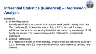
data shows the number of patients who are not regularly taking medications
however it does not explain why. Collecting qualitative data through interviews
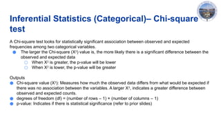
and analyzing it may reveal that cost barriers or painful side effects are reasons
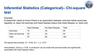
why patients are not regularly taking medications.
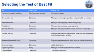
5.
What is QuantitativeData Analysis?
This presentation focuses on quantitative data analysis which is the process of
analyzing numerical information to better understand relationships between
variables.
● Focuses on statistical analysis to better assess trends and patterns
● Useful to better explain the “what” of global public health issues
● Applies to both:
○ Categorical (qualitative) data – ex. gender, occupation, blood type
○ Numerical (quantitative) data – ex. age, blood pressure, heart rate
● Most analyses are performed using statistical software (ex. R, STATA, SAS,
and so forth).
6.
Example 2
A researcheris interested in seeing if the high blood pressure medication (from
example 1) is effective. Measuring systolic and diastolic blood pressure before
treatment and after 6 months of treatment will allow for quantitative comparison
and analysis to determine whether the medication works.
7.
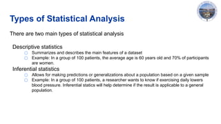
Types of StatisticalAnalysis
There are two main types of statistical analysis
Descriptive statistics
○ Summarizes and describes the main features of a dataset
○ Example: In a group of 100 patients, the average age is 60 years old and 70% of participants
are women.
Inferential statistics
○ Allows for making predictions or generalizations about a population based on a given sample
○ Example: In a group of 100 patients, a researcher wants to know if exercising daily lowers
blood pressure. Inferential statics will help determine if the result is applicable to a general
population.
8.
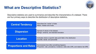
What are DescriptiveStatistics?
•Describes the “center” of data
•Mean, median and mode
Central Tendency
•Spread of values in the dataset
•Range, variance, and standard deviation
Dispersion
•Indicates where a specific data point falls in the distribution
•Quartile, decile, and percentile
Location
•Summarizes how often something happens
•Proportion, rate, prevalence, incidence, odds ratio (OR), and relative risk (RR)
Proportions and Rates
Descriptive statistics are used to summarize and describe the characteristics of a dataset. There
are four primary ways to describe the distribution of descriptive statistics.
9.
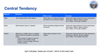
Central Tendency
Measure Definition
Whento Use Example
Mean
The average value of the dataset When data is normally distributed
and there are no extreme outliers
Heart rate measurements from five participants
are 60 bpm, 90bpm, 80bpm, 80bpm,
and 110bpm. The mean is 84bpm.
Mode Most frequent value in a dataset When evaluating categorical data
(nominal)
Heart rate measurements from five participants
are 60 bpm, 90bpm, 80bpm, 80bpm,
and 110bpm. The mode is 80bpm
Median Midpoint (or middle) value in a dataset
.
Data should be arranged in ascending
order.
• If the number of values is odd, the
median is the middle number.
• If even, it is the average of the two
middle numbers.
When data is skewed or has
outliers
Heart rate measurements from five participants
are 60 bpm, 80 bpm, 80 bpm, 90bpm,
and 110bpm. The median is 80 bpm
bpm indicates “beats per minute”, which is the heart rate
10.
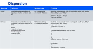
Dispersion
Measure Definition Whento Use Example
Range Shows the difference between the
largest and smallest number in data
set
For a quick glance
at variability of dataset
Heart rate measurements from five participants are 60 bpm, 90bpm,
80bpm, 80bpm, and 110bpm.
110 bpm – 60 bpm = 50 bpm
The range is 50bpm
Variance
Variance demonstrates how closely
the dataset is spread in relation to the
mean.
Where:
= sample variance
= number of data points
= each data point
= sample mean
Statistical modeling
or comparing variability
Heart rate measurements from five participants are 60 bpm, 90bpm,
80bpm, 80bpm, and 110bpm.
1) Calculate the mean ():
=
=
2) Find squared differences from the mean:
=
=
=
=
=
3) Sum of squared differences:
4) Divide by
=
=
The variance is 330 bpm
11.
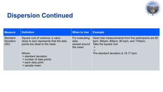
Dispersion Continued
Measure DefinitionWhen to Use Example
Standard
Deviation
(SD)
Square root of variance; a value
close to zero represents that the data
points are close to the mean
Where:
= standard deviation
= number of data points
= each data point
= sample mean
For evaluating
data
spread around
the mean
Heart rate measurements from five participants are 60
bpm, 90bpm, 80bpm, 80 bpm, and 110bpm.
Take the square root
=
=
The standard deviation is 18.17 bpm
12.
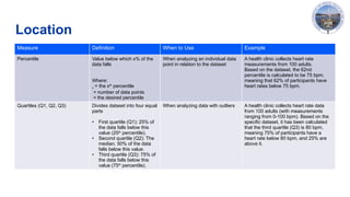
Location
Measure Definition Whento Use Example
Percentile Value below which x% of the
data falls
Where:
x = the xth
percentile
= number of data points
= the desired percentile
When analyzing an individual data
point in relation to the dataset
A health clinic collects heart rate
measurements from 100 adults.
Based on the dataset, the 62nd
percentile is calculated to be 75 bpm,
meaning that 62% of participants have
heart rates below 75 bpm.
Quartiles (Q1, Q2, Q3) Divides dataset into four equal
parts
• First quartile (Q1): 25% of
the data falls below this
value (25th
percentile).
• Second quartile (Q2): The
median. 50% of the data
falls below this value.
• Third quartile (Q3): 75% of
the data falls below this
value (75th
percentile).
When analyzing data with outliers A health clinic collects heart rate data
from 100 adults (with measurements
ranging from 0-100 bpm). Based on the
specific dataset, it has been calculated
that the third quartile (Q3) is 80 bpm,
meaning 75% of participants have a
heart rate below 80 bpm, and 25% are
above it.
13.
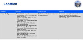
Location
Measure Definition Whento Use Example
Deciles (D1– D10) Divides data into ten parts
• First decile (D1): 10% of the data falls
below this value.
• Second decile (D2): 20% of the data
falls below this value.
• Third decile (D3): 30% of the data falls
below this value.
• Fourth decile (D4): 40% of the data
falls below this value.
• Fifth decile (D5): 50% of the data falls
below this value. The median.
• Sixth decile (D6): 60% of the data falls
below this value.
• Seventh decile (D7): 70% of the data
falls below this value.
• Eighth decile (D8): 80% of the data
falls below this value.
• Ninth decile (D9): 90% of the data falls
below this value.
Similar to quartiles, but more beneficial
for larger datasets
In the same dataset, it has been calculated
that the ninth decile (D9) is 85 bpm,
meaning 90% of participants have a heart
rate below 85 bpm.
14.
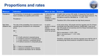
Proportions and rates
MeasureDefinition When to Use Example
Prevalence
The proportion of individuals in a population who
have a condition at a specific point in time
Prevalence =
To describe how
common a
disease or
condition is within
a population.
A health clinic surveys 200 adults. A researcher finds that 60
adults within the survey population have high blood pressure. The
prevalence would be calculated as x (100) = 30%
Therefore 30% of the sample has high blood pressure.
Risk Ratio
(Relative risk)
The ratio of the probability of an outcome in an
exposed group compared to an unexposed
group.
RR =
=
Where:
• a = # with outcome in exposed group
• b = # without outcome in exposed group
• c = # with outcome in unexposed group
• d= # without outcome in unexposed group
If…
RR = 1: there is no association
RR > 1: exposure increases risk for disease
RR < 1: exposure decreases risk for disease
In cohort
studies or clinical
trials to
compare risk bet
ween two groups.
In the same study, 100 people exercise regularly and 20 of these
individuals have high blood pressure. Additionally, it was found
that 100 people do not exercise and 40 of these individuals have
high blood pressure.
Risk in exercisers= = 0.20 = 20%
Risk in non-exercisers = = 0.5 = 40%
RR = = 0.5
Therefore, individuals who exercise regularly have half the risk of
developing high blood pressure compared to those who don’t.
15.
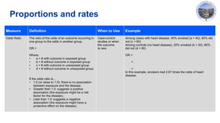
Proportions and rates
MeasureDefinition When to Use Example
Odds Ratio The ratio of the odds of an outcome occurring in
one group to the odds in another group.
OR =
Where:
• a = # with outcome in exposed group
• b = # without outcome in exposed group
• c = # with outcome in unexposed group
• d = # without outcome in unexposed group
If the odds ratio is…
• 1.0 (or close to 1.0): there is no association
between exposure and the disease.
• Greater than 1.0: suggests a positive
association (the exposure might be a risk
factor for the disease).
• Less than 1.0: suggests a negative
association (the exposure might have a
protective effect on the disease).
Case-control
studies or when
the outcome
is rare.
Among cases with heart disease, 40% smoked (a = 40), 60% did
not (c = 60)
Among controls (no heart disease), 20% smoked (b = 20), 80%
did not (d = 80)
OR =
=
=
In this example, smokers had 2.67 times the odds of heart
disease.
16.
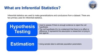
What are InferentialStatistics?
• Used to assess if there is enough evidence to reject the null
hypothesis.
• The null hypothesis (H ) is a statement that there is no effect or
₀
difference. It represents the assumption a researcher is trying to
test against.
Hypothesis
Testing
• Using sample data to estimate population parameters
Estimation
Inferential statistics are used to make generalizations and conclusions from a dataset. There are
two primary uses for inferential statistics.
17.
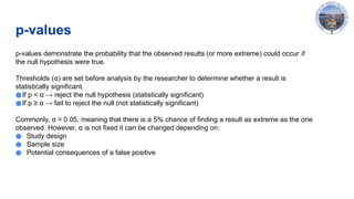
p-values
p-values demonstrate theprobability that the observed results (or more extreme) could occur if
the null hypothesis were true.
Thresholds (α) are set before analysis by the researcher to determine whether a result is
statistically significant.
●If p < α → reject the null hypothesis (statistically significant)
●If p ≥ α → fail to reject the null (not statistically significant)
Commonly, α = 0.05, meaning that there is a 5% chance of finding a result as extreme as the one
observed. However, α is not fixed it can be changed depending on:
● Study design
● Sample size
● Potential consequences of a false positive
18.
p-values
Example:
A researcher isstudying whether a new heart medication lowers blood pressure compared to a
placebo.
After analyzing the data, they find:
• p = 0.03
• α = 0.05 (set by researcher)
Interpretation:
Since p = 0.03 (which means p < 0.05), the result is statistically significant. This means there is
only a 3% probability that the observed difference (or a more extreme one) occurred by chance
if the medication had no true effect. The researcher rejects the null hypothesis (the new
medication causes no difference) and concludes that the new medication likely lowers blood
pressure.
19.
Confidence Intervals
A confidenceinterval (CI) provides a range of values that likely contains
the true population value (such as the true mean or proportion), based on
the sample data.
Interpretation depends on the confidence level (commonly 95%):
• A 95% CI means that if we repeated the study many times, 95% of the
intervals would contain the true value.
• 99% CI is used when consequences of a wrong conclusion are high. It
provides greater certainty, but the interval will be wider.
• 90% CI is used where a narrower range is acceptable and a quicker
decision is needed.
20.
Confidence Intervals
Example:
Guo andZhang (2017) evaluated the association between ideal
cardiovascular health (CVH) metrics and risk of cardiovascular events as
well as mortality. When looking at smoking as an ideal CVH metric, they
found that the risk ratio was RR = 0.54 (95% CI: 0.38-0.77) with p = 0.001
for cardiovascular mortality.
Interpretation:
Ideal smoking status (non-smoking) is associated with a 46% lower risk of
dying from cardiovascular causes. This is shown by a risk ratio (RR) of
0.54 with a 95% confidence interval from 0.38 to 0.77, meaning we are
95% confident that the true effect falls in this range.
21.
Inferential Statistics (Numerical)– Pearson
Correlation Coefficient
Pearson Correlation Coefficient: a statistical test that measures the strength
and direction of a linear relationship between two continuous variables.
Pearson correlation coefficient is denoted by r
○ Ranges from -1 to +1
○ r = -1 a perfect negative linear relationship
○ r = +1 a perfect positive linear relationship
○ r = 0 no linear relationship
22.
Inferential Statistics (Numerical)– Pearson
Correlation Coefficient
Example:
Reimers et al. (2018), studied whether regular exercise influences resting
heart rate (RHR). They reported a correlation of r = -0.36 between baseline
RHR and the change of RHR after participating in different types of sports.
This indicates that individuals with higher baseline RHR tend to show a
decrease in RHR after participating in a sport.
23.
Inferential Statistics (Numerical)– Student’s
t-test
Types of t-tests:
• 1-sample t-test: comparing the mean of one group to a known value
• 2-sample t-test: evaluating two independent groups
• 2-sample paired t-test: using the same group at two different time points
Outputs from a t-test:
• t-value: Size of the difference relative to variability in the sample data. A larger value
indicates that there is a greater difference between groups.
• Degrees of freedom (df): Number of independent variables that vary with respect to a given
analysis. Affects the shape of t-distribution.
• p-value: Shows the probability that the observed difference is due to chance (if p < 0.05)
A Student’s t-test compares the means of two groups or of one group to determine if they are
significantly different. Certain assumptions must be met to use a t-test (normality, independent
observations, similar variances, and random sampling).
24.
Inferential Statistics (Numerical)– Student’s
t-test
Example: Paired t-test
A researcher wants to know if a walking program reduces resting heart rate (RHR). 50 adults are
measured before and after the program.
○ Before: mean RHR = 78 bpm
○ After: mean RHR = 72 bpm
○ Standard deviation of differences = 4 bpm
A paired t-test is conducted:
○ t = 7.07: The difference between the before and after RHR is large relative to the variability in
the data.
○ df = 49: Degrees of freedom (50 participants – 1).
○ p < 0.001: There is less than a 0.1% chance that the result is due to random variation.
Since p < 0.05, the difference is statistically significant. Therefore, the walking program significantly
reduced RHR.
25.
Inferential Statistics (Numerical)– ANOVA
Analysis of Variance (ANOVA) evaluates the means of more than two groups to
see if the mean across the groups is statistically significant
● There are three primary types of ANOVA
1) One-way ANOVA: One independent variable being assessed
2) Two-way ANOVA: Two independent variables being assessed
3) Repeated Measures ANOVA: Same group measured multiple times
In ANOVA, independent variables are compared based on their effect on
a dependent variable, which must be quantitative (numerical).
26.
Inferential Statistics (Numerical)– ANOVA
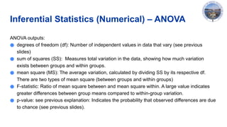
ANOVA outputs:
● degrees of freedom (df): Number of independent values in data that vary (see previous
slides)
● sum of squares (SS): Measures total variation in the data, showing how much variation
exists between groups and within groups.
● mean square (MS): The average variation, calculated by dividing SS by its respective df.
There are two types of mean square (between groups and within groups)
● F-statistic: Ratio of mean square between and mean square within. A large value indicates
greater differences between group means compared to within-group variation.
● p-value: see previous explanation: Indicates the probability that observed differences are due
to chance (see previous slides).
27.
Inferential Statistics (Numerical)– ANOVA
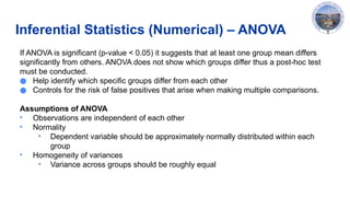
If ANOVA is significant (p-value < 0.05) it suggests that at least one group mean differs
significantly from others. ANOVA does not show which groups differ thus a post-hoc test
must be conducted.
● Help identify which specific groups differ from each other
● Controls for the risk of false positives that arise when making multiple comparisons.
Assumptions of ANOVA
• Observations are independentof each other
• Normality
• Dependent variable should be approximately normally distributed within each
group
• Homogeneity of variances
• Variance across groups should be roughly equal
28.
Inferential Statistics (Numerical)– ANOVA
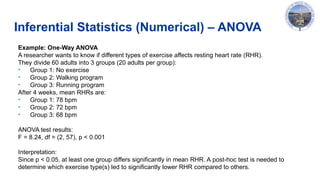
Example: One-Way ANOVA
A researcher wants to know if different types of exercise affects resting heart rate (RHR).
They divide 60 adults into 3 groups (20 adults per group):
• Group 1: No exercise
• Group 2: Walking program
• Group 3: Running program
After 4 weeks, mean RHRs are:
• Group 1: 78 bpm
• Group 2: 72 bpm
• Group 3: 68 bpm
ANOVA test results:
F = 8.24, df = (2, 57), p < 0.001
Interpretation:
Since p < 0.05, at least one group differs significantly in mean RHR. A post-hoc test is needed to
determine which exercise type(s) led to significantly lower RHR compared to others.
29.
Inferential Statistics (Numerical)– Regression
Analysis
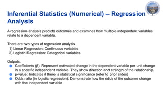
A regression analysis predicts outcomes and examines how multiple independent variables
relate to a dependent variable.
There are two types of regression analysis
1) Linear Regression: Continuous variables
2) Logistic Regression: Categorical variables
Outputs:
● Coefficients (β): Represent estimated change in the dependent variable per unit change
in a specific independent variable. They show direction and strength of the relationship.
● p-value: Indicates if there is statistical significance (refer to prior slides)
● Odds ratio (in logistic regression): Demonstrate how the odds of the outcome change
with the independent variable
30.
Inferential Statistics (Numerical)– Regression
Analysis
Examples
● Linear Regression:
A study examined how hours of exercise per week predict resting heart rate.
The coefficient (β) for exercise was –1.8 (p < 0.01). In short, for every
additional hour of exercise, resting heart rate decreased by an average of 1.8
beats per minute. The p-value indicates this relationship is statistically
significant.
● Logistic Regression:
In a regression model on heart disease, smokers had an odds ratio of 2.5 (p =
0.02). Smokers were 2.5 times more likely than non-smokers to develop heart
disease.
31.
Inferential Statistics (Categorical)–Chi-square
test
A Chi-square test looks for statistically significant association between observed and expected
frequencies among two categorical variables.
● The larger the Chi-square (X2
) value is, the more likely there is a significant difference between the
observed and expected data
○ When X2
is greater, the p-value will be lower
○ When X2
is lower, the p-value will be greater
Outputs
● Chi-square value (X2
): Measures how much the observed data differs from what would be expected if
there was no association between the variables. A larger X2
, indicates a greater difference between
observed and expected counts.
● degrees of freedom (df) = (number of rows – 1) × (number of columns – 1)
● p-value: Indicates if there is statistical significance (refer to prior slides)
32.
Inferential Statistics (Categorical)–Chi-square
test
Example:
A researcher wants to know if there is an association between exercise habits (exercises
regularly vs. does not exercise) and heart disease status (has heart disease vs. does not).
Heart Disease No Heart Disease Total
Exercises 10 40 50
Does not exercise 30 20 50
Total 40 60 100
Chi-square test provides: X2
= 6.63, df = 1, p = 0.01
Interpretation: Since p < 0.05, a conclusion can be made that exercise habits are significantly
associated with heart disease status.
33.
Selecting the Testof Best Fit
Test Type of Data When to Use
Pearson’s correlation coefficient Two continuous variables Correlation analysis
One-sample t-test Continuous When you have one group and are comparing it to an average
Independent t-test Continuous When you are comparing two separate groups
Paired t-test Continuous When you are measuring one group twice
One-way ANOVA Continuous When you are analyzing the means of more than two groups
Two-way ANOVA Continuous When you are analyzing the means of more than two groups and
have two independent variables
Repeated Measures ANOVA Continuous When you are evaluating the same group at multiple time points
Linear regression Continuous Model relationships
Logistic regression Binary When you have binary/dichotomous variables
Chi-square test Categorical Comparing proportions
34.
References
● Aguinis, H.,Vassar, M., & Wayant, C. (2019). On reporting and interpreting statistical significance and P values in
medical research. BMJ Evidence-Based Medicine, 26(2), 39–42. https://doi.org/10.1136/bmjebm-2019-111264
● Buderer, N. M., & Brannan, G. (2024, May 19). Comparing the means of independent groups: ANOVA, Ancova,
MANOVA, and Mancova. StatPearls [Internet]. https://www.ncbi.nlm.nih.gov/sites/books/NBK606084/
● The Chi squared tests. The BMJ. (2021, April 12).
https://www.bmj.com/about-bmj/resources-readers/publications/statistics-square-one/8-chi-squared-tests
● Faizi, N., & Alvi, Y. (2023). Correlation. Biostatistics Manual for Health Research, 109–126.
https://doi.org/10.1016/b978-0-443-18550-2.00002-5
● Government of Canada. (2021, September 2). Measures of Dispersion. Statistics Canada.
https://www150.statcan.gc.ca/n1/edu/power-pouvoir/ch12/5214891-eng.htm
● Green, J. L., Manski, S. E., Hansen, T. A., & Broatch, J. E. (2023). Descriptive statistics. International Encyclopedia
of Education(Fourth Edition), 723–733. https://doi.org/10.1016/b978-0-12-818630-5.10083-1
● Guo, L., & Zhang, S. (2017). Association between Ideal Cardiovascular Health Metrics and risk of cardiovascular
events or mortality: A meta analysis of prospective studies.
‐ Clinical Cardiology, 40(12), 1339–1346.
https://doi.org/10.1002/clc.22836
● Holt, M. (2022). Statistical dispersion. EBSCO. https://www.ebsco.com/research-starters/science/statistical-
dispersion
● Kotronoulas, G., Miguel, S., Dowling, M., Fernández-Ortega, P., Colomer-Lahiguera, S., Bağçivan, G., Pape, E.,
Drury, A., Semple, C., Dieperink, K. B., & Papadopoulou, C. (2023). An overview of the fundamentals of data
management, analysis, and Interpretation in Quantitative Research. Seminars in Oncology Nursing, 39(2), 151398.
https://doi.org/10.1016/j.soncn.2023.151398
35.
References
● LibreTexts. (2020,August 11). Measures of location. Statistics LibreTexts.
https://stats.libretexts.org/Courses/Las_Positas_College/Math_40%3A_Statistics_and_Probability/
03%3A_Data_Description/3.03%3A_Measures_of_Position/3.3.01%3A_Measures_of_Location-_Deciles
● Marshall, G., & Jonker, L. (2011). An introduction to inferential statistics: A review and practical
guide. Radiography, 17(1). https://doi.org/10.1016/j.radi.2009.12.006
● McDermid, R. (2021). Statistics in medicine. Anaesthesia & Intensive Care Medicine, 22(7), 454–462.
https://doi.org/10.1016/j.mpaic.2021.05.009
● McHugh, M. L. (2013). The chi-square test of Independence. Biochemia Medica, 143–149.
https://doi.org/10.11613/bm.2013.018
● Measures of central tendency. Australian Bureau of Statistics. (n.d.-a).
https://www.abs.gov.au/statistics/understanding-statistics/statistical-terms-and-concepts/measures-central-tendency
● Measures of shape. Australian Bureau of Statistics. (n.d.-b). https://www.abs.gov.au/statistics/understanding-
statistics/statistical-terms-and-concepts/measures-shape
● Mohr, D. L., Wilson, W. J., & Freund, R. J. (2022). Linear regression. Statistical Methods, 301–349.
https://doi.org/10.1016/b978-0-12-823043-5.00007-2
● National Institutes of Health. (n.d.). Finding and using health statistics. U.S. National Library of Medicine.
https://www.nlm.nih.gov/oet/ed/stats/02-900.html
● Reimers, A. K., Knapp, G., & Reimers, C.-D. (2018). Effects of exercise on the resting heart rate: A systematic
review and meta-analysis of Interventional Studies. Journal of Clinical Medicine, 7(12), 503.
https://doi.org/10.3390/jcm7120503
36.
References
● Runeson, P.(2016). Mere numbers aren’t enough. Perspectives on Data Science for Software Engineering, 303–
307. https://doi.org/10.1016/b978-0-12-804206-9.00055-6
● Salas-Parra, R. D., Castro-Ochoa, K. J., & Machado-Aranda, D. A. (2023). Basic science statistics. Translational
Surgery, 195–199. https://doi.org/10.1016/b978-0-323-90300-4.00022-7
● Shreffler, J., & Huecker, M. (2023, March 13). Hypothesis testing, P values, confidence intervals, and
significance. StatPearls [Internet]. https://www.ncbi.nlm.nih.gov/books/NBK557421/
● Smalheiser, N. R. (2017). ANOVA. Data Literacy, 149–155. https://doi.org/10.1016/b978-0-12-811306-6.00011-7
● Tenny, S., Brannan, J., & Brannan, G. (2022, September 18). Qualitative study. StatPearls [Internet].
https://www.ncbi.nlm.nih.gov/books/NBK470395/
● Wadhwa, R. R., & Azzam, D. (2023, July 17). Variance. StatPearls [Internet].
https://www.ncbi.nlm.nih.gov/books/NBK551689/
● Wadhwa, R. R., & Marappa-Ganeshan, R. (2023, January 16). T test. StatPearls [Internet].
https://www.ncbi.nlm.nih.gov/books/NBK553048/
● Wert, J. E., Neidt, C. O., & Ahmann, J. S. (1954). Quartiles, deciles, and percentiles. Statistical Methods in
Educational and Psychological Research., 39–49. https://doi.org/10.1037/11779-003
● World Health Organization. (2019). Using qualitative research to strengthen guideline development. World Health
Organization. https://www.who.int/news/item/08-08-2019-using-qualitative-research-to-strengthen-guideline-
development