Chapter 4 a

CHAPTER IV
FINDINGS AND ANALYSIS
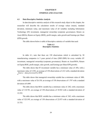
4.1

Data Descriptive Statistics Analysis
In data descriptive statistics analysis of this research study object in this chapter, the

researcher will describe the calculation results of average values (mean), standard
deviation, minimum value, and maximum value of all variables including Information
Technology (IT) investment, managerial ownership (corporate governance), Return on
Asset (ROA), Return on Equity (ROE), profit margin, sales growth and Earnings per Share
(EPS) growth.
The table shown below is table of descriptive statistics of variable that used:
Table 4.1
Descriptive Statistics

In table 4.1, note that there are 150 observations which is calculated by 30
manufacturing companies in 5 years period of time (2005-2009) for every variable (IT
investment, managerial ownership (corporate governance), Return on Asset/ROA, Return
on Equity/ROE, profit margin, sales growth, and Earnings per Share/EPS growth).
The table shows that IT investment variable has a minimum value of .056, with a
maximum value of 2.292, an average of 150 observations of .612 with a standard deviation
Source : data processed by SPSS
of .457.
The table shows that managerial ownership variable has a minimum value of .000,
with a maximum value of 26.150, an average of 150 observations of 1.797 with a standard
deviation of 6.009.
The table shows that ROA variable has a minimum value of .202, with a maximum
value of 110.781, an average of 150 observations of 10.922 with a standard deviation of
12.252.
The table shows that ROE variable has a minimum value of .543, with a maximum
value of 323.595, an average of 150 observations of 22.073 with a standard deviation of
33.753.

24

The table shows that profit margin variable has a minimum value of .003, with a
maximum value of 1.000, an average of 150 observations of .087 with a standard deviation
of .116.
The table shows that sales growth variable has a minimum value of -.476, with a
maximum value of .658, an average of 150 observations of .168 with a standard deviation
of .184.
The table shows that EPS growth variable has a minimum value of -.858 with a
maximum value of 19.500, an average of 150 observations of .571 with a standard
deviation of 1.931.
4.2

Data Normality Test
The method in testing data normality test was done by using the P-P Plot test by

comparing the plot of cumulative distribution of the normal distribution that forms a
straight line compared to the plots of residual data, and if the plot of the residual data were
around the diagonal line, it can conclude that the data are normally distributed (Ghozali,
2001). If the data plot are scattered around diagonal line then the regression model is valid
for normality assumption. Besides that, if data plots are scattered far with the diagonal line
then the regression model is invalid for normality assumption.
There two basics decision making in analyzing P-P Plot test:
a. If the data are spread around the diagonal line and follow the direction of
diagonal lines, then it can conclude that the regression model meets the
assumption of normality.
b. If the data are spread too far from the diagonal line and not follow the direction
of the diagonal line, then it can conclude that the regression model does not
meet the assumption of normality.
There are the results of data normality test using P-P Plot test:

25

Normal P-P Plot of ROA
1.0

Expected Cum Prob

0.8

0.6

0.4

0.2

0.0
0.0

0.2

0.4

0.6

0.8

1.0

Observed Cum Prob
Transforms: natural log

Figure 4.1
Normality Test Result of Return on Asset (ROA)
Normal P-P Plot of ROE
1.0

Expected Cum Prob

0.8

0.6

0.4

0.2

0.0
0.0

0.2

0.4

0.6

0.8

1.0

Observed Cum Prob

Figure 4.2
Normality Test Result of Return on Equity (ROE)

26

Normal P-P Plot of PROFIT MARGIN
1.0

Expected Cum Prob

0.8

0.6

0.4

0.2

0.0
0.0

0.2

0.4

0.6

0.8

1.0

Observed Cum Prob

Figure 4.3
Normality Test Result of Profit Margin
Normal P-P Plot of SALES GROWTH
1.0

Expected Cum Prob

0.8

0.6

0.4

0.2

0.0
0.0

0.2

0.4

0.6

0.8

1.0

Observed Cum Prob

Figure 4.4
Normality Test Result of Sales Growth

27

Normal P-P Plot of EPS GROWTH
1.0

Expected Cum Prob

0.8

0.6

0.4

0.2

0.0
0.0

0.2

0.4

0.6

0.8

1.0

Observed Cum Prob

Figure 4.5
Normality Test Result of Earnings per Share (EPS) Growth
Normal P-P Plot of MANAGERIAL OWNERSHIP
1.0

Expected Cum Prob

0.8

0.6

0.4

0.2

0.0
0.0

0.2

0.4

0.6

0.8

1.0

Observed Cum Prob

Figure 4.6
Normality Test Result of Managerial Ownership (Corporate Governance)

28

Normal P-P Plot of IT INVESTMENT
1.0

Expected Cum Prob

0.8

0.6

0.4

0.2

0.0
0.0

0.2

0.4

0.6

0.8

1.0

Observed Cum Prob

Figure 4.7
Normality Test Result of IT Investment
Based on seven figures above, it clearly shows that all plots of the residual data is
around the diagonal line, it means the data are spread around the diagonal line and follow
the direction of diagonal lines, thus it can be concluded that all the data are normally
distributed. In addition, all figures are results of data processed by SPSS.
4.3

Classical Assumption Test
Before conducting hypothesis test using multiple regression testing, classical

assumption test violations test is needed for the model that used in this research study.
Classical assumption test used to ensure that the multiple regression models is not bias so
that the result of estimates or predictions can be trusted, for the multiple regression
equation used multicollinearity test, autocorrelation test and heteroscedasticity test.
4.3.1

Multicollinearity Test
Multicollinearity test shows that each the independent variables have a

strong direct relationship (correlation), the value of Variance Infatuations Factor
(VIF) and tolerance used to detect whether there is any multicollinearity or not
(Ghozali, 2001).

29

Moreover, when value of Variance Infatuations Factor (VIF) is less than 10
or Tolerance (TOL) is more than 0,1 it can be concluded that there is no
multicollinearity.
Ho : there is no multicollinearity
Ha : there is a multicollinearity
a. If VIF < 10 or TOL > 0,1, Ho is accepted
b. If VIF > 10 or TOL > 0,1, Ho is rejected
Table 4.2
Multicollinearity Test Result
a
Coefficients

Model
1

(Constant)
MANAGERIAL
OWNERSHIP
IT INVESTMENT

Unstandardized
Coefficients
B
Std. Error
13.852
.989

Standardized
Coefficients
Beta

t
14.002

Sig.
.000

Collinearity Statistics
Tolerance
VIF

-2.225

.628

-.268

-3.543

.001

.997

1.003

-5.241

1.248

-.317

-4.199

.000

.997

1.003

a. Dependent Variable: ROA

Based on the table 4.2, VIF value shows 1.003 and Tolerance value shows .
997 that represent all dependent variables to all independent variables, it is known
that each independent variable used in this research study has VIF value less than
10 and tolerance value more than 0.10, it can be concluded that the regression
model has no multicollinearity problems.
4.3.2

Autocorrelation Test
Autocorrelation test indicates that there is a correlation between the errors in

one period with the error of the previous period which is in the classical assumption
test, this case should not happen. Autocorrelation test is done by using the Durbin
Watson method (Ghozali, 2001). Autocorrelation test steps performed as follows:
Ho : there is no autocorrelation
Ha : there is an autocorrelation
There are four basics decisions making of autocorrelation test:
a. If the DW value is located between the upper limit or upper bound (du)
and (4-du), then the autocorrelation coefficient equal to zero, it means
there is no autocorrelation.

30

b. If the DW value is lower than the lower limit or lower bound (dl), then
the autocorrelation coefficient is greater than zero, it means there is
positive autocorrelation.
c. If the DW value is greater than the (4-dl), then the autocorrelation
coefficient is smaller than zero, it means there is a negative
autocorrelation, and
d. If the DW value is located between the upper limit (du) and the lower
limit (dl) or DW is located between (4-du) and (4-dl), the results are
inconclusive.
Table 4.3
Autocorrelation Test Decisions
Criteria
0 < DW <dl
dl < DW < du
4-dl < DW < 4

Ho
Rejected
Inconclusive
Rejected

Decisions
There is positive autocorrelation
Inconclusive
There is negative autocorrelation

4-du < DW < 4-dl
du < DW < 4-du

Inconclusive
Accepted

Inconclusive
There is no autocorrelation

Table 4.4
Autocorrelation Test Results (n = 150 , k’ = 5 )
Equation 1 Return on Asset (ROA)
b
Model Summary

Model
1

R
.404a

Adjusted
R Square
.151

R Square
.163

Std. Error of
the Estimate
6.950483

DurbinWatson
2.075

a. Predictors: (Constant), IT INVESTMENT, MANAGERIAL OWNERSHIP
b. Dependent Variable: ROA
There is

There is

There is no

positive

Inconclusive

autocorrelation

autocorrelation

negative

Inconclusive

autocorrelation

Inconclusive

dl

du

4-du

4-dl

1.706

1.760

2.240

2.294

DW

Conclusion

2.075


31

0
0

dl
1.70

du

DW

4-du

4-dl

4

1.760

2.075

2.240

2.294

4

Based on the table 4.4, the lower limit (dl) is known from the Durbin
Watson table for n = 150 and k = 5 at a significant level of 5% is 1.706 and the
upper limit value (du) is the 1.760, value of Durbin Watson for 2.075 is in the du ≤
dw ≤ 4-du area, it means there is no autocorrelation in the regression model.
Table 4.5
Equation 2 Return on Equity (ROE)
b
Model Summary

Model
1

R
.356a

R Square
.127

Adjusted
R Square
.115

Std. Error of
the Estimate
12.573854

DurbinWatson
1.989

b. Dependent Variable: ROE

There is
positive

Inconclusive

autocorrelation

dl
0 1.706
0

There is

There is no
autocorrelation

Inconclusive

autocorrelation

Inconclusive

du

4-du

1.760
dl

2.240
du

1.706

negative

1.760

4-dl

DW

2.294
1.989
DW
1.989

Conclusion
4-du
4-dl
4
2.240

2.294

4

Table 4.6
Equation 3 Profit Margin

32

b
Model Summary

Model
1

R
.296a

Adjusted
R Square
.075

R Square
.088

Std. Error of
the Estimate
.053205

DurbinWatson
2.133

b. Dependent Variable: PROFIT MARGIN

There is

There is

There is no

positive

Inconclusive

autocorrelation

autocorrelation

negative

Inconclusive

autocorrelation

Inconclusive

0

dl

du

DW

4-du

4-dl

4

0

1.706

1.760

2.133

2.240

2.294

4

dl

du

4-du

4-dl

DW

Conclusion

1.706

1.760

2.240

2.294

2.133


Table 4.7
Equation 4 Sales Growth

33

b
Model Summary

Model
1

R
.063a

Adjusted
R Square
-.010

R Square
.004

Std. Error of
the Estimate
.184676

DurbinWatson
1.838

b. Dependent Variable: SALES GROWTH


There is

There is

There is no

positive

Inconclusive

autocorrelation

autocorrelation

negative

Inconclusive

autocorrelation

Inconclusive

0

dl

du

DW

4-du

4-dl

4

0

1.706

1.760

1.838

2.240

2.294

4

dl

du

4-du

4-dl

DW

Conclusion

1.706

1.760

2.240

2.294

1.838


Table 4.8
Equation 5 Earnings per Share (EPS) Growth

34

There is
positive

Inconclusive

autocorrelation

There is

There is no
autocorrelation

negative

Inconclusive

autocorrelation

Inconclusive

0

dl

du

DW

4-du

4-dl

4

0

1.706

1.760

1.806

2.240

2.294

4

b
Model Summary

Model
1

R
.062a

R Square
.004

Adjusted
R Square
-.010

Std. Error of
the Estimate
.667276

DurbinWatson
1.806

b. Dependent Variable: EPS GROWTH

dl

du

4-du

4-dl

DW

Conclusion

1.706

1.760

2.240

2.294

1.838


35

Based on five autocorrelation test results above, the data in this research
study was known in the decision that there is no autocorrelation in the regression
model, so the regression model that used can be continued.
4.3.3

Heteroscedasticity Test
Heteroscedasticity test indicates that the variance of each error is

heterogeneous which means that violate the classical assumption which requires
that the variance of the error must be homogeneous (Ghozali, 2001).
Heteroscedasticity test by Spearman Rank test is to correlate the independent
variables with the residual value. Heteroscedasticity test is used to analyst whether
all variants errors are hetero or homo.
Heteroscedasticity test steps performed as follows:
Ho: There is no heteroscedasticity
Ha: There is a heteroscedasticity

There are two basics decisions making of heteroscedasticity test:
a. If p-value > 0.05 then Ho is accepted (there is no
heteroscedasticity)
b. If

p-value

<

0.05

then

Ho

is

rejected

(there

is

a

heteroscedasticity)
Table 4.9
Heteroscedasticity test result with Spearman Rank for ROA
Correlations

Spearman's rho

Unstandardized Residual

MANAGERIAL
OWNERSHIP
IT INVESTMENT

Correlation Coefficient
Sig. (2-tailed)
N
Sig. (2-tailed)
N
Sig. (2-tailed)
N

36

Unstandardiz
ed Residual
1.000
.
150
-.023
.781
150
.039
.636
150

MANAGERIAL
OWNERSHIP
-.023
.781
150
1.000
.
150
-.099
.227
150

IT
INVESTMENT
.039
.636
150
-.099
.227
150
1.000
.
150

Based on the table 4.9 are known that each independent variable has a pvalue more than 0.05. Managerial ownership (corporate governance) with p-value
of .781, IT investment with p-value of .636 which means that there is no
heteroscedasticity problem in the regression model.
Table 4.10
Heteroscedasticity test with Spearman Rank for ROE
Correlations

Spearman's rho


MANAGERIAL
OWNERSHIP
IT INVESTMENT

Sig. (2-tailed)
N
Sig. (2-tailed)
N
Sig. (2-tailed)
N

Unstandardiz
ed Residual
1.000
.
150
-.075
.359
150
.044
.592
150

MANAGERIAL
OWNERSHIP
-.075
.359
150
1.000
.
150
-.099
.227
150

IT
INVESTMENT
.044
.592
150
-.099
.227
150
1.000
.
150

Table 4.11
Heteroscedasticity test result with Spearman Rank for Profit Margin
Correlations

Spearman's rho


MANAGERIAL
OWNERSHIP
IT INVESTMENT

Sig. (2-tailed)
N
Sig. (2-tailed)
N
Sig. (2-tailed)
N

Unstandardiz
ed Residual
1.000
.
150
-.004
.965
150
.025
.762
150

MANAGERIAL
OWNERSHIP
-.004
.965
150
1.000
.
150
-.099
.227
150

IT
INVESTMENT
.025
.762
150
-.099
.227
150
1.000
.
150

37

Table 4.12
Heteroscedasticity test result with Spearman Rank for Sales Growth
Correlations

Spearman's rho


MANAGERIAL
OWNERSHIP
IT INVESTMENT

Sig. (2-tailed)
N
Sig. (2-tailed)
N
Sig. (2-tailed)
N

Unstandardiz
ed Residual
1.000
.
150
.005
.954
150
-.032
.698
150

MANAGERIAL
OWNERSHIP
.005
.954
150
1.000
.
150
-.099
.227
150

IT
INVESTMENT
-.032
.698
150
-.099
.227
150
1.000
.
150


Table 4.13
Heteroscedasticity test result with Spearman Rank for EPS Growth
Correlations

Spearman's rho


MANAGERIAL
OWNERSHIP
IT INVESTMENT

Sig. (2-tailed)
N
Sig. (2-tailed)
N
Sig. (2-tailed)
N

Unstandardiz
ed Residual
1.000
.
150
-.063
.445
150
-.018
.829
150

MANAGERIAL
OWNERSHIP
-.063
.445
150
1.000
.
150
-.099
.227
150

IT
INVESTMENT
-.018
.829
150
-.099
.227
150
1.000
.
150

38

4.4

Hypothesis Test
Hypothesis test is analyzed by seeing the significance value of each relationship.

Level of significance (α) is set at 5%, which means the error limit that can be tolerated is
5%. It means the level of confidence in testing this hypothesis is 95%. If p-value < 0.05, it
can be concluded that the independent variables have a significant relationship with
dependent variables.
Firstly, there is the result of coefficient determination test between IT investments
and managerial ownership (corporate governance) as independent variables toward ROA as
dependent variable:
Table 4.14
Coefficient Determination Test Results of ROA
b
Model Summary

Model
1

R
.404a

R Square
.163

Adjusted
R Square
.151

Std. Error of
the Estimate
6.950483

DurbinWatson
2.075


From the table 4.14, it shows that the coefficient (R) is .404. It means that the
correlation or relationship between independent variables, IT investment and managerial
ownership (corporate governance), and ROA as dependent variable is not significant
because of the correlation values < 0.50.
While the value of Adjusted R Square (coefficient of determination) is .151 which
means that ROA can be explained by independent variables, IT investment and managerial
ownership (corporate governance), amounted to .151 or by 15.1% while the remaining
balance of 84.9% explained by other factors which are not included in this research study.
Secondly, there is the result of coefficient determination test between IT
investments and managerial ownership (corporate governance) as independent variables
toward ROE as dependent variable:
Table 4.15
Coefficient Determination Test Result of ROE
39

b
Model Summary

Model
1

R
.356a

R Square
.127

Adjusted
R Square
.115

Std. Error of
the Estimate
12.573854

DurbinWatson
1.989


ownership (corporate governance), and ROE as dependent variable is not significant
means that ROE can be explained by independent variables, IT investment and managerial
Thirdly, there is the result of coefficient determination test between IT investments
and managerial ownership (corporate governance) as independent variables toward profit
margin as dependent variable:

Table 4.16
Coefficient Determination Test Results of Profit Margin
b
Model Summary

Model
1

R
.296a

R Square
.088

Adjusted
R Square
.075

Std. Error of
the Estimate
.053205

DurbinWatson
2.133

Source :Dependent Variable: PROFIT MARGIN
b. data processed by SPSS

ownership (corporate governance), and profit margin as dependent variable is not
significant because of the correlation values < 0.50.
40

means that profit margin can be explained by independent variables, IT investment and
managerial ownership (corporate governance), amounted to .075 or by 7.5% while the
remaining balance of 92.5% explained by other factors which are not included in this
research study.
Fourthly, there is the result of coefficient determination test between IT investments
and managerial ownership (corporate governance) as independent variables toward sales
growth as dependent variable:
Table 4.17
Coefficient Determination Test Result of Sales Growth
b
Model Summary

Model
1

R
.063a

R Square
.004

Adjusted
R Square
-.010

Std. Error of
the Estimate
.184676

DurbinWatson
1.838


ownership (corporate governance), and sales growth as dependent variable is not significant
relationship because of the correlation values < 0.50.
While the value of R Square (coefficient of determination) is .004 which means that
sales growth can be explained by independent variables, IT investment and managerial
Fifthly, there is the result of coefficient determination test between IT investments
and managerial ownership (corporate governance) as independent variables toward EPS
growth as dependent variable:
Table 4.18
Coefficient Determination Test Result of EPS Growth

41

b
Model Summary

Model
1

R
.062a

R Square
.004

Adjusted
R Square
-.010

Std. Error of
the Estimate
.667276

DurbinWatson
1.806


ownership (corporate governance), and EPS growth as dependent variable is not significant
While the value of R Square (coefficient of determination) is .004 which means that
EPS growth can be explained by independent variables, IT investment and managerial
Table 4.8

Table 4.19
Results Summary of Hypothesis Test for IT Investment
Variable

ROA

ROE

Profit Margin

42

Sales Growth

EPS Growth

Constant
R2
Coefissien B
T stat
Sig.
Conclusion

13.852
.151
-5.241
-4.199
.000
Ha is

25.088
.115
-8.585
-3.802
.000
Ha is rejected

.083
.075
-.002
-.157
.875
Ha is

.252
.004
.084
.702
.484
Ha is

accepted

rejected

.169
.004
.007
.203
.840
Ha is
accepted

accepted

Table 4.20
Results Summary of Hypothesis Test for Managerial Ownership
Variable

ROA

Constant
R2
Coefissien B
T stat
Sig.
Conclusion

13.852
.151
-2.225
-3.543
.001
Ha is

ROE

Profit Margin

Sales Growth

EPS Growth

.169
.004
-.012
-.731
.466
Ha is

.252
.004
-.013
-.220
.826
Ha is

accepted

accepted

25.088
.083
.115
.075
-3.218
-.018
-2.832
-3.757
.005
.000
Ha is rejected Ha is rejected

rejected

T-Test Results (Multiple Regression) of ROA
a
Coefficients

Model
1

(Constant)
MANAGERIAL
OWNERSHIP
IT INVESTMENT

Unstandardized
Coefficients
B
Std. Error
13.852
.989

Standardized
Coefficients
Beta

t
14.002

Sig.
.000

Tolerance
VIF

-2.225

.628

-.268

-3.543

.001

.997

1.003

-5.241

1.248

-.317

-4.199

.000

.997

1.003

a. Dependent Variable: ROA

Hypothesis 1a
The first hypothesis tested the relationship of IT investment to ROA. There is the
hypothesis prepared as follows:
H1a : There is significant relationship between IT investment and ROA
43

Based on the table 4.8, it can be concluded that IT investment do not affect ROA with a
significance level of .000, it means the significant level is < 0.05 and t count -4.199 then ttable
-1.9761, it means -4.199 > -1.9761, it can be concluded that H 1a is rejected and it means
that IT investment do not significantly affect ROA.
Hypothesis 3a
The second hypothesis tested the relationship of managerial ownership to ROA. There is
the hypothesis prepared as follows:
H3a : There is significant relationship between managerial ownership and ROA
Based on the table 4.8, it can be concluded that managerial ownership do not affect ROA
with a significance level of .001, it means the significant level is < 0.05 and t count -3.543
then ttable -1.9761, it means -3.543 > -1.9761, it can be concluded that H 3a is rejected and it
means that managerial ownership do not significantly affect ROA.
Table 4.9
T-Test Results (Multiple Regression) of ROE
a
Coefficients

Model
1

(Constant)
MANAGERIAL
OWNERSHIP
IT INVESTMENT

Unstandardized
Coefficients
B
Std. Error
25.088
1.790

Standardized
Coefficients
Beta

t
14.018

Sig.
.000

Tolerance
VIF

-3.218

1.136

-.219

-2.832

.005

.997

1.003

-8.585

2.258

-.294

-3.802

.000

.997

1.003

a. Dependent Variable: ROE

Hypothesis 1b
The third hypothesis tested the relationship of IT investment to ROE. There is the
H1b : There is significant relationship between IT investment and ROE
Based on the table 4.9, it can be concluded that IT investment do not affect ROE with a
significance level of .000, it means the significant level is < 0.05 and t count -3.802 then ttable
-1.9761, it means -3.802 > -1.9761, it can be concluded that H1b is rejected and it means
that IT investment do not significantly affect ROE.
Hypothesis 3b
The fourth hypothesis tested the relationship of managerial ownership to ROE. There is the
H3b : There is significant relationship between managerial ownership and ROE
44

Based on the table 4.9, it can be concluded that managerial ownership do not affect ROE
with a significance level of .005, it means the significant level is < 0.05 and t count -2.832
then ttable -1.9761, it means -2.832 > -1.9761, it can be concluded that H3b is rejected and it
means that managerial ownership do not significantly affect ROE.
Table 4.10
T-Test Results (Multiple Regression) of Profit Margin
a
Coefficients

Model
1

(Constant)
MANAGERIAL
OWNERSHIP
IT INVESTMENT

Unstandardized
Coefficients
B
Std. Error
.083
.008

Standardized
Coefficients
Beta

t
10.954

Sig.
.000

Tolerance
VIF

-.018

.005

-.296

-3.757

.000

.997

1.003

-.002

.010

-.012

-.157

.875

.997

1.003

a. Dependent Variable: PROFIT MARGIN

Hypothesis 1c
The fifth hypothesis tested the relationship of IT investment to profit margin. There is the
H1c : There is significant relationship between IT investment and profit margin
Based on the table 4.10, it can be concluded that IT investment affects profit margin with a
significance level of .875, it means the significant level is > 0.05 and t count -.157 then ttable
-1.9761, it means -.157 < -1.9761, it can be concluded that H 1c is accepted and it means that
IT investment significantly affects profit margin.
Hypothesis 3c
The sixth hypothesis tested the relationship of managerial ownership to profit margin.
There is the hypothesis prepared as follows:
H3c : There is significant relationship between managerial ownership and profit margin
Based on the table 4.10, it can be concluded that managerial ownership do not affect profit
margin with a significance level of .000, it means the significant level is < 0.05 and t count
-3.757 then ttable -1.9761, it means -3.757 > -1.9761, it can be concluded that H3c is rejected
and it means that managerial ownership do not significantly affect profit margin.
Table 4.11
T-Test Results (Multiple Regression) of Sales Growth

45

a
Coefficients

Model
1

(Constant)
MANAGERIAL
OWNERSHIP
IT INVESTMENT

Unstandardized
Coefficients
B
Std. Error
.169
.026

Standardized
Coefficients
Beta

t
6.421

Sig.
.000

Tolerance
VIF

-.012

.017

-.060

-.731

.466

.997

1.003

.007

.033

.017

.203

.840

.997

1.003

a. Dependent Variable: SALES GROWTH

Hypothesis 2a
The seventh hypothesis tested the relationship of IT investment to sales growth. There is
the hypothesis prepared as follows:
H2a : There is significant relationship between IT investment and sales growth
Based on the table 4.11, it can be concluded that IT investment affects sales growth with a
significance level of .840, it means the significant level is > 0.05 and t count .203 then ttable
1.9761, it means .203 < 1.645, it can be concluded that H 2a is accepted and it means that IT
investment significantly affects sales growth.
Hypothesis 4a
The eighth hypothesis tested the relationship of managerial ownership to profit margin.
There is the hypothesis prepared as follows:
H4a : There is significant relationship between managerial ownership and sales growth
Based on the table 4.11, it can be concluded that managerial ownership affects profit
margin with a significance level of .466, it means the significant level is > 0.05 and t count
-.731 then ttable -1.9761, it means -.731 < -1.9761, it can be concluded that H 4a is accepted
and it means that managerial ownership significantly affects sales growth.
Table 4.12
T-Test Results (Multiple Regression) With EPS Growth
a
Coefficients

Model
1

(Constant)
MANAGERIAL
OWNERSHIP
IT INVESTMENT

Unstandardized
Coefficients
B
Std. Error
.252
.095

Standardized
Coefficients
Beta

t
2.653

Sig.
.009

Tolerance
VIF

-.013

.060

-.018

-.220

.826

.997

1.003

.084

.120

.058

.702

.484

.997

1.003

a. Dependent Variable: EPS GROWTH

Hypothesis 2b
The ninth hypothesis tested the relationship of IT investment to EPS growth. There is the
H2b : There is significant relationship between IT investment and EPS growth

46

Based on the table 4.12, it can be concluded that IT investment affects EPS growth with a
significance level of .484, it means the significant level is > 0.05 and t count .702 then ttable
1.9761, it means .702 < 1.9761, it can be concluded that H 2b is accepted and it means that
IT investment significantly affects EPS growth.
Hypothesis 4b
The tenth hypothesis tested the relationship of managerial ownership to EPS growth. There
is the hypothesis prepared as follows:
H4b : There is significant relationship between managerial ownership and EPS growth
Based on the table 4.12, it can be concluded that managerial ownership affects EPS growth
with a significance level of .826, it means the significant level is > 0.05 and t count -.220 then
ttable -1.9761, it means -.220 < -1.9761, it can be concluded that H 4b is accepted and it means
that managerial ownership significantly affects EPS growth.
Table 4.13
F (ANOVA) Test Result of ROA
b
ANOVA

Model
1

Regression
Residual
Total

Sum of
Squares
1381.156
7101.455
8482.611

df
2
147
149

Mean Square
690.578
48.309

F
14.295

Sig.
.000a


Hypothesis 5a
This hypothesis is tested to see the relationship of IT investment and managerial
ownership (corporate governance) to ROA in the same time.
H5a : IT investment and managerial ownership have a significant relationship toward ROA
in the same time.
The table 4.13 shows that Fcount is 14.295 which higher than Ftable 3.06 and pvalue is .
000 which lower than 0.05, it can be concluded that H 5a is accepted and it means IT
investment and managerial ownership have a significant relationship toward ROA in the
same time.
Table 4.14
F (ANOVA) Test Result of ROE
47

ANOVAb
Model
1

Regression
Residual
Total

Sum of
Squares
3371.141
23240.964
26612.105

df

Mean Square
1685.570
158.102

2
147
149

F
10.661

Sig.
.000a


Hypothesis 5b
ownership toward ROE in the same time.
H5b : IT investment and managerial ownership have a significant relationship toward ROE
in the same time.
000 which lower than 0.05, it can be concluded that H 5b is accepted and it means IT
investment and managerial ownership have a significant relationship toward ROE in the
same time.
Table 4.15
F (ANOVA) Test Result of Profit Margin
ANOVAb
Model
1

Regression
Residual
Total

Sum of
Squares
.040
.416
.456

df
2
147
149

Mean Square
.020
.003

F
7.060

Sig.
.001a

b. Dependent Variable: PROFIT MARGIN

Hypothesis 5c
ownership toward profit margin in the same time.
H5c : IT investment and managerial ownership have a significant relationship toward profit
margin in the same time.

48

000 which lower than 0.05, it can be concluded that H 5c is accepted and it means IT
investment and managerial ownership have a significant relationship toward profit margin
in the same time.

Table 4.16
F (ANOVA) Test Result of Sales Growth
ANOVAb
Model
1

Regression
Residual
Total

Sum of
Squares
.020
5.013
5.034

df

Mean Square
.010
.034

2
147
149

F
.297

Sig.
.744a


Hypothesis 5d
ownership toward sales growth in the same time.
H5d : IT investment and managerial ownership have a significant relationship toward sales
growth in the same time.
The table 4.16 shows that Fcount is .297 which lower than F table 3.06 and pvalue is .744
which higher than 0.05, it can be concluded that H5d is rejected and it means IT investment
and managerial ownership have not significant relationship toward ROA in the same time.
Table 4.17
F (ANOVA) Test Result of EPS Growth
b
ANOVA

Model
1

Regression
Residual
Total

Sum of
Squares
.250
65.453
65.703

df
2
147
149

Mean Square
.125
.445

F
.280


Hypothesis 5e
49

Sig.
.756a

ownership toward EPS growth in the same time.
H5e : IT investment and managerial ownership have a significant relationship toward EPS
growth in the same time.
The table 4.17 shows that Fcount is .280 which lower than Ftable 3.06 and pvalue is .756 which
higher than 0.05, it can be concluded that H 5e is rejected and it means IT investment and
managerial ownership have not significant relationship toward ROA in the same time.

50

Chapter 4 a

Recommended

Recommended

More Related Content

Similar to Chapter 4 a

Similar to Chapter 4 a (20)

Recently uploaded

Recently uploaded (20)

Chapter 4 a