Linear Regression (Machine Learning)

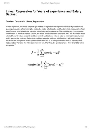
1. 9/17/2019 ML_Activity_1 - Jupyter Notebook
localhost:8890/notebooks/ML Activity/ML_Activity_1.ipynb 1/12
Linear Regression for Years of experience and Salary
Dataset
Gradient Descent in Linear Regression
In linear regression, the model targets to get the best-fit regression line to predict the value of y based on the
given input value (x). While training the model, the model calculates the cost function which measures the Root
Mean Squared error between the predicted value (pred) and true value (y). The model targets to minimize the
cost function. To minimize the cost function, the model needs to have the best value of θ1 and θ2. Initially model
selects θ1 and θ2 values randomly and then itertively update these value in order to minimize the cost function
untill it reaches the minimum. By the time model achieves the minimum cost function, it will have the best θ1
and θ2 values. Using these finally updated values of θ1 and θ2 in the hypothesis equation of linear equation,
model predicts the value of x in the best manner it can. Therefore, the question arises – How θ1 and θ2 values
get updated ?

2. 9/17/2019 ML_Activity_1 - Jupyter Notebook
localhost:8890/notebooks/ML Activity/ML_Activity_1.ipynb 2/12

3. 9/17/2019 ML_Activity_1 - Jupyter Notebook
localhost:8890/notebooks/ML Activity/ML_Activity_1.ipynb 3/12
-> θj : Weights of the hypothesis. -> hθ(xi) : predicted y value for ith input. -> j : Feature index number (can be 0,
1, 2, ......, n). -> α : Learning Rate of Gradient Descent. We graph cost function as a function of parameter
estimates i.e. parameter range of our hypothesis function and the cost resulting from selecting a particular set
of parameters. We move downward towards pits in the graph, to find the minimum value. Way to do this is
taking derivative of cost function as explained in the above figure. Gradient Descent step downs the cost
function in the direction of the steepest descent. Size of each step is determined by parameter α known as
Learning Rate.
In the Gradient Descent algorithm, one can infer two points :
1.If slope is +ve : θj = θj – (+ve value). Hence value of θj decreases.

4. 9/17/2019 ML_Activity_1 - Jupyter Notebook
localhost:8890/notebooks/ML Activity/ML_Activity_1.ipynb 4/12
2. If slope is -ve : θj = θj – (-ve value). Hence value of θj increases.
The choice of correct learning rate is very important as it ensures that Gradient Descent converges in a
reasonable time. :
1.If we choose α to be very large, Gradient Descent can overshoot the minimum.
It may fail to converge or even diverge.
2.If we choose α to be very small, Gradient Descent will take small steps to reach
local minima and will take a longer time to reach minima.
For linear regression Cost Function graph is always convex shaped.
Reference: geeksforgeeks.org/gradient-descent-in-linear-regression/ (Refered
For Theory)

5. 9/17/2019 ML_Activity_1 - Jupyter Notebook
localhost:8890/notebooks/ML Activity/ML_Activity_1.ipynb 5/12
First, we import a few libraries-
In [10]:
Data Preprocessing & importing Dataset
The next step is to import our dataset ‘Salary_Data.csv’ then split them into input (independent) variables and
output (dependent) variable. When you deal with real datasets, you usually have around thousands of rows but
since the one I have taken here is a sample, this has just 30 rows. So when we split our data into a training set
and a testing set, we split it in 1/3, i.e., 20 rows go into the training set and the rest 10 make it to the testing set.
In [11]:
Plotting Default Dataset
Out[11]:
YearsExperience Salary
0 1.1 39343.0
1 1.3 46205.0
2 1.5 37731.0
3 2.0 43525.0
4 2.2 39891.0
import numpy as np
import pandas as pd
import matplotlib.pyplot as plt
dataset = pd.read_csv('Salary_Data.csv')
x = dataset.iloc[:, :-1].values
y = dataset.iloc[:, 1].values
data_top = dataset.head() #Dataset display
data_top

6. 9/17/2019 ML_Activity_1 - Jupyter Notebook
localhost:8890/notebooks/ML Activity/ML_Activity_1.ipynb 6/12
In [12]:
Training & Split
Split arrays or matrices into random train and test subsets
In [13]:
Linear Regression
Now, we will import the linear regression class, create an object of that class, which is the linear regression
model.
In [14]:
Fitting Data
Then we will use the fit method to “fit” the model to our dataset. What this does is nothing but make the
regressor “study” our data and “learn” from it.
plt.scatter(x, y, color = "red")
plt.plot(x,y, color = "green")
plt.title("Salary vs Experience (Dataset)")
plt.xlabel("Years of Experience")
plt.ylabel("Salary")
plt.show()
from sklearn.model_selection import train_test_split
x_train, x_test, y_train, y_test = train_test_split(x, y, test_size = 1/3)
from sklearn.linear_model import LinearRegression
lr = LinearRegression()

7. 9/17/2019 ML_Activity_1 - Jupyter Notebook
localhost:8890/notebooks/ML Activity/ML_Activity_1.ipynb 7/12
In [15]:
Testing
Now that we have created our model and trained it, it is time we test the model with our testing dataset.
In [16]:
Data Visualization for Training Dataset
First, we make use of a scatter plot to plot the actual observations, with x_train on the x-axis and y_train on the
y-axis. For the regression line, we will use x_train on the x-axis and then the predictions of the x_train
observations on the y-axis. We add a touch of aesthetics by coloring the original observations in red and the
regression line in green.
In [17]:
Data Visualization for Testing Dataset
repeat the same task for our testing dataset, and we get the following code-
Out[15]:
LinearRegression(copy_X=True, fit_intercept=True, n_jobs=None, normalize=Fal
se)
lr.fit(x_train, y_train)
y_pred = lr.predict(x_test)
plt.scatter(x_train, y_train, color = "red")
plt.plot(x_train, lr.predict(x_train), color = "green")
plt.title("Salary vs Experience (Training set)")
plt.xlabel("Years of Experience")
plt.ylabel("Salary")
plt.show()

8. 9/17/2019 ML_Activity_1 - Jupyter Notebook
localhost:8890/notebooks/ML Activity/ML_Activity_1.ipynb 8/12
In [24]:
Linear Regression with Gradient Descent Algorithm
Approach for Years of experience and Salary
Dataset
Importing libraries,Dataset & data preprocessing
plt.scatter(x_test, y_test, color = "red")
plt.plot(x_train, lr.predict(x_train), color = "green")
plt.title("Salary vs Experience (Testing set)")
plt.xlabel("Years of Experience")
plt.ylabel("Salary")
plt.show()

9. 9/17/2019 ML_Activity_1 - Jupyter Notebook
localhost:8890/notebooks/ML Activity/ML_Activity_1.ipynb 9/12
In [27]:
# Making the imports
import numpy as np
import pandas as pd
import matplotlib.pyplot as plt
plt.rcParams['figure.figsize'] = (12.0, 9.0)
# Preprocessing Input data
data = pd.read_csv('Salary_Data.csv')
X = data.iloc[:, 0]
Y = data.iloc[:, 1]
#Plotting Data for visualization
plt.scatter(X, Y)
plt.title("Salary vs Experience (Dataset set)")
plt.xlabel("Years of Experience")
plt.ylabel("Salary")
plt.show()

10. 9/17/2019 ML_Activity_1 - Jupyter Notebook
localhost:8890/notebooks/ML Activity/ML_Activity_1.ipynb 10/12
Optimizing parameter value like intercept "c" and slope "m" & learning rate
alpha in Gradient descent formula
In [26]:
Prediction
Slope & Intercept:
12836.600965885045 2915.2044856014018
# Building the model
m = 0
c = 0
L = 0.0001 # The learning Rate
#L = 0.0001 # The learning Rate
#L = 0.0002 # The learning Rate
#L = 0.0003 # The learning Rate
epochs = 1000 # The number of iterations to perform gradient descent
n = float(len(X)) # Number of elements in X
# Performing Gradient Descent
for i in range(epochs):
Y_pred = m*X + c # The current predicted value of Y
D_m = (-2/n) * sum(X * (Y - Y_pred)) # Derivative wrt m
D_c = (-2/n) * sum(Y - Y_pred) # Derivative wrt c
m = m - L * D_m # Update m
c = c - L * D_c # Update c
print("Slope & Intercept:")
print (m, c)

11. 9/17/2019 ML_Activity_1 - Jupyter Notebook
localhost:8890/notebooks/ML Activity/ML_Activity_1.ipynb 11/12
In [28]:
# Making predictions
Y_pred = m*X + c
plt.scatter(X, Y)
plt.plot([min(X), max(X)], [min(Y_pred), max(Y_pred)], color='red') # regression line
plt.title("Salary vs Experience (prediction)")
plt.xlabel("Years of Experience")
plt.ylabel("Salary")
plt.show()

12. 9/17/2019 ML_Activity_1 - Jupyter Notebook
localhost:8890/notebooks/ML Activity/ML_Activity_1.ipynb 12/12
Batch 1 Block 1 B.TECH ENTC
Omkar Rane BETB118
Kaustubh Wankhade BETB129