Farmers can produce crops using different combinations of capital and labor. In the US, crops are typically grown using capital-intensive technology, while in developing countries crops are grown using more labor-intensive production. Isoquants can show the different options for crop production using different amounts of capital and labor.

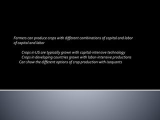
1. Farmers can produce crops with different combinations of capital and labor
of capital and labor
Crops in US are typically grown with capital-intensive technology
Crops in developing countries grown with labor-intensive productions
Can show the different options of crop production with isoquants

2. 2
INTERNAL EVALUATION
Assignment and group work in class 5
Case Study 5
Test/CP Forum 5
15 ( Pre-mid)
Mid term 20 (50)
Post mid term (Assignment) 10
Group Presentation 5
Test 5
CP /Attendance 5
25 (Post-mid)
End Semester 40 (100)

3. 3
Main Topics on which questions can arise
What do you mean by Law ofVariable Proportions?
Short run production function?
Caselet: Call Centre
Which is the ideal stage of production?
What do you understand by Law of Diminishing returns
Caselet: Healthcare in US- Production function
What is an Isoquant and mention its properties? Elaborate on Isocost line?
What are the two types of producers equilibrium?And conditions
Caselet Energy and other inputs Isoquant and Isocost
Returns to scale – Elaborate
Caselet :Carpet industry in US
What are the different types of cost concepts- Elaborate
Behaviour of the short term cost concepts(TFC,TVC,TC,MC&
AC,AVC,AFC)

4. Long run average cost curves - Elaborate
Why is the LRAC U shaped / What do you mean by economies and diseconomies
Of scale?
What do you mean by economies to scale and economies of scope?
Caselet:
Elaborate on Break even point and shut down point?
Case: DishTV

5. Chapter 6 5
Capital
Labor
250 500 760 1000
40
80
120
100
90
Output = 13,800 bushels
per year
A
10
-
K 

B
260
L 

Point A is more
capital-intensive, and
B is more labor-intensive.

6. opportunity cost Cost associated with opportunities that are
forgone when a firm’s resources are not put to their best
alternative use.
economic cost Cost to a firm of utilizing economic resources in
production, including opportunity cost
accounting cost Actual expenses plus depreciation charges
for capital equipment.
MEASURING COST:

7. The Northwestern University Law School has been located in Chicago. However, the
main campus is located in the suburb of Evanston.
In the mid-1970s, the law school began planning the construction of a new building
and needed to decide on an appropriate location.
Should it be built on the current site, near downtown Chicago law firms?
Should it be moved to Evanston, physically integrated with the rest of the university?
Some argued it was cost-effective to locate the new building in the city because the
university already owned the land. Land would have to be purchased in Evanston if
the building were to be built there.
Does this argument make economic sense?
No. It makes the common mistake of failing to appreciate opportunity costs. From an
economic point of view, it is very expensive to locate downtown because the property
could have been sold for enough money to buy the Evanston land with substantial
funds left over.
Northwestern decided to keep the law school in Chicago.

8. MEASURING COST:
Fixed Costs andVariable Costs
total cost (TC or C) Total economic cost of production,
consisting of fixed and variable costs.
TFC+TVC =TC
fixed cost (FC) Cost that does not vary with the level
of output and that can be eliminated only by shutting
down.
variable cost (VC) Cost that varies as output varies.
The only way that a firm can eliminate its fixed costs is by shutting
down.

9. Sunk Costs
● sunk cost Expenditure that has
been made and cannot be
recovered.
Because a sunk cost cannot be recovered, it should not
influence the firm’s decisions.
For example, consider the purchase of specialized
equipment for a plant. Suppose the equipment can be used
to do only what it was originally designed for and cannot be
converted for alternative use. The expenditure on this
equipment is a sunk cost. Because it has no alternative use,
its opportunity cost is zero. Thus it should not be included as
part of the firm’s economic costs.

10. Marginal Cost (MC)
● marginal cost (MC) Increase in cost resulting from
the production of one extra unit of output.
Because fixed cost does not change as the firm’s level of output changes,
marginal cost is equal to the increase in variable cost or the increase in
total cost that results from an extra unit of output.
We can therefore write marginal cost as

11. Fixed Costs and Variable Costs
Shutting Down
Shutting down doesn’t necessarily mean going out of business.
By reducing the output of a factory to zero, the company could eliminate the
costs of raw materials and much of the labor. The only way to eliminate fixed
costs would be to close the doors, turn off the electricity, and perhaps even sell
off or scrap the machinery.
Fixed or Variable
How do we know which costs are fixed and which are variable?
Over a very short time horizon—say, a few months—most costs are fixed.
Over such a short period, a firm is usually obligated to pay for contracted
shipments of materials.
Over a very long time horizon—say, ten years—nearly all costs are variable.
Workers and managers can be laid off (or employment can be reduced by
attrition), and much of the machinery can be sold off or not replaced as it
becomes obsolete and is scrapped.

12. Fixed versus Sunk Costs
Amortizing Sunk Costs
amortization Policy of treating a
one-time expenditure as an annual
cost spread out over some number of
years.
Sunk costs are costs that have been incurred and cannot be
recovered.
An example is the cost of R&D to a pharmaceutical company to
develop and test a new drug and then, if the drug has been
proven to be safe and effective, the cost of marketing it.
Whether the drug is a success or a failure, these costs cannot be
recovered and thus are sunk.

13. It is important to understand the characteristics of production costs and to be able to
identify which costs are fixed, which are variable, and which are sunk.
Good examples include the personal computer industry (where most costs are
variable), the computer software industry (where most costs are sunk), and the
pizzeria business (where most costs are fixed).
Because computers are very similar, competition is intense, and profitability
depends on the ability to keep costs down. Most important are the variable cost of
components and labor.
A software firm will spend a large amount of money to develop a new application.
The company can try to recoup its investment by selling as many copies of the
program as possible.
For the pizzeria, sunk costs are fairly low because equipment can be resold if the
pizzeria goes out of business. Variable costs are low—mainly the ingredients for
pizza and perhaps wages for a couple of workers to help produce, serve, and
deliver pizzas.

14. Marginal andAverage Cost
TABLE 7.1 A Firm’s Costs
Rate of Fixed Variable Total Marginal Average Average Average
Output Cost Cost Cost Cost Fixed Cost Variable Cost Total Cost
(Units (Dollars (Dollars (Dollars (Dollars (Dollars (Dollars (Dollars
per Year) per Year) per Year) per Year) per Unit) per Unit) per Unit) per Unit)
(FC) (VC) (TC) (MC) (AFC) (AVC) (ATC)
(1) (2) (3) (4) (5) (6) (7)
0 50 0 50 -- -- -- --
1 50 50 100 50 50 50 100
2 50 78 128 28 25 39 64
3 50 98 148 20 16.7 32.7 49.3
4 50 112 162 14 12.5 26 36
6 50 150 200 20 8.3 25 33.3
7 50 175 225 25 28 40.5
5 50 130 180 18 10 7.1 25 32.1
8 50 204 254 29 6.3 25.5 31.8
9 50 242 292 38 5.6 26.9 32.4
10 50 300 350 58 5 30 35
11 50 385 435 85 4.5 35 39.5
Marginal Cost (MC)

15. Average Total Cost (ATC)
average total cost (ATC) Firm’s total cost divided by its
level of output
TC/Q
AFC+AVC
.
average fixed cost (AFC) Fixed cost divided by the level of
output.
TFC/Q
average variable cost (AVC) Variable cost divided by the level of
output.
TVC/Q

16. The Shapes of the Cost Curves
In (a) total cost TC is the
vertical sum of fixed cost
FC and variable cost VC.
In (b) average total cost
ATC is the sum of
average variable cost
AVC and average fixed
cost AFC.
Marginal cost MC crosses
the average variable cost
and average total cost
curves at their minimum
points.

17. Diminishing marginal returns means that the marginal product of labor
declines as the quantity of labor employed increases.
As a result, when there are diminishing marginal returns, marginal cost
will increase as output increases.
Diminishing Marginal Returns and Marginal Cost
The change in variable cost is the per-unit cost of the extra labor w times
the amount of extra labor needed to produce the extra output ΔL. Because
ΔVC = wΔL, it follows that
The extra labor needed to obtain an extra unit of output is ΔL/Δq =
1/MPL. As a result,

18. Choosing Inputs
Facing an isocost curve
C1, the firm produces
output q1 at point A using
L1 units of labor and K1
units of capital.
When the price of labor
increases, the isocost
curves become steeper.
Output q1 is now
produced at point B on
isocost curve C2 by using
L2 units of labor and K2
units of capital.

19. Choosing Inputs
Recall that in our analysis of production technology, we showed
that the marginal rate of technical substitution of labor for
capital (MRTS) is the negative of the slope of the isoquant and
is equal to the ratio of the marginal products of labor and
capital:
It follows that when a firm minimizes the cost of producing a particular
output, the following condition holds:
We can rewrite this condition slightly as follows:

20. Long-Run AverageCost
When a firm is producing at
an output at which the long-
run average cost LAC is
falling, the long-run marginal
cost LMC is less than LAC.
Conversely, when LAC is
increasing, LMC is greater
than LAC.
The two curves intersect at A,
where the LAC curve
achieves its minimum.

21. Long-Run AverageCost
long-run average cost curve (LAC) Curve
relating average cost of production to output
when all inputs, including capital, are variable.
short-run average cost curve (SAC) Curve
relating average cost of production to output when
level of capital is fixed.
long-run marginal cost curve (LMC) Curve
showing the change in long-run total cost as
output is increased incrementally by 1 unit.

22. Economies and Diseconomies of Scale
As output increases, the firm’s average cost of producing that output
is likely to decline, at least to a point.
This can happen for the following reasons:
1. If the firm operates on a larger scale, workers can specialize
in the activities at which they are most productive.
2. Scale can provide flexibility. By varying the combination of
inputs utilized to produce the firm’s output, managers can
organize the production process more effectively.
3. The firm may be able to acquire some production inputs at
lower cost because it is buying them in large quantities and
can therefore negotiate better prices. The mix of inputs
might change with the scale of the firm’s operation if
managers take advantage of lower-cost inputs.

23. Diseconomies of Scale
At some point, however, it is likely that the average cost of
production will begin to increase with output.
There are three reasons for this shift:
1. At least in the short run, factory space and machinery may
make it more difficult for workers to do their jobs effectively.
2. Managing a larger firm may become more complex and
inefficient as the number of tasks increases.
3. The advantages of buying in bulk may have disappeared
once certain quantities are reached. At some point,
available supplies of key inputs may be limited, pushing
their costs up.

24. economies of scale Situation in which output can be
doubled for less than a doubling of cost.
diseconomies of scale Situation in which a doubling
of output requires more than a doubling of cost.
Increasing Returns to Scale: Output more than doubles when
the quantities of all inputs are
doubled.
Economies of Scale: A doubling of output requires less
than a doubling of cost.

25. The Relationship Between Short-Run and Long-Run Cost
The long-run average cost curve
LAC is the envelope of the short-
run average cost curves SAC1,
SAC2, and SAC3.
With economies and diseconomies
of scale, the minimum points of the
short-run average cost curves do
not lie on the long-run average cost
curve. (Envelope curve)

26. Economies of scope is an economic concept that the unit cost to produce a
product will decline as the variety of products increases.That is, the more
different-but-similar goods you produce, the lower the total cost to produce each
one.
For example, let’s say that you’re a shoe manufacturer.You produce men’s and
women’s sneakers. Adding a children’s line of sneakers would increase economies
of scope because you can use the same production equipment, supplies, storage,
and distribution channels to make a new line of products.That will further reduce
the cost of production on all your shoes.
The cost to produce all three of your different lines is lower than if three
different companies each produced a line of men’s shoes, a line of women’s
shoes, and a children’s line
Economies to Scope Vs economies to scale

27. Economies of Scale
You’ve probably heard of economies of scale, which is a similar economic concept
– but not exactly. Economies of scale are gained simply by producing more
products – through more volume. So if you were a necklace manufacturer,
you could reduce the cost per piece by producing more necklaces. As
production increases, the average cost per unit declines.
n contrast, with economies of scope, you need to produce more different types of
products using the same resources.
So instead of producing more necklaces, you would also produce bracelets and
rings and earrings and charms, for example.You would add new types of products
that could be produced with the same equipment and materials in order to reduce
your average costs.

28. BREAK EVEN ANALYSIS
Break Even Analysis in economics, business, and cost accounting refers to the point in
which total cost and total revenue are equal. A break even point analysis is used to
determine the number of units or dollars of revenue needed to cover total costs (fixed
and variable costs).
Break even quantity = Fixed costs / (Sales price per unit –Variable cost per unit)
Where:
Fixed costs are costs that do not change with varying output (e.g., salary, rent, building
machinery).
Sales price per unit is the selling price (unit selling price) per unit.
Variable cost per unit is the variable costs incurred to create a unit.
It is also helpful to note that sales price per unit minus variable cost per unit is
the contribution margin per unit. For example, if a book’s selling price is $100 and its
variable costs are $5 to make the book, $95 is the contribution margin per unit and
contributes to offsetting the fixed costs.

29. Example of Break Even Analysis
Colin is the managerial accountant in charge of Company A, which sells water bottles. He
previously determined that the fixed costs of Company A consist of property taxes, a lease,
and executive salaries, which add up to $100,000.The variable cost associated with
producing one water bottle is $2 per unit.The water bottle is sold at a premium price of
$12.To determine the break even point of Company A’s premium water bottle:
Break even quantity = $100,000 / ($12 – $2) = 10,000
Therefore, given the fixed costs, variable costs, and selling price of the water bottles,
Company A would need to sell 10,000 units of water bottles to break even.

30. Graphically Representing the Break Even Point
The graphical representation of unit sales and dollar sales needed to break even is
referred to as the break even chart or CostVolume Profit (CVP) graph. Below is the
CVP graph of the example above:

31. Explanation:
The number of units is on the X-axis (horizontal) and the dollar amount is on theY-axis (vertical).
The red line represents the total fixed costs of $100,000.
The blue line represents revenue per unit sold. For example, selling 10,000 units would generate
10,000 x $12 = $120,000 in revenue.
The yellow line represents total costs (fixed and variable costs). For example, if the company
sells 0 units, then the company would incur $0 in variable costs but $100,000 in fixed costs for
total costs of $100,000. If the company sells 10,000 units, the company would incur 10,000 x
$2 = $20,000 in variable costs and $100,000 in fixed costs for total costs of $120,000.
The break even point is at 10,000 units. At this point, revenue would be 10,000 x $12 = $120,000
and costs would be 10,000 x 2 = $20,000 in variable costs and $100,000 in fixed costs.
When the number of units exceeds 10,000, the company would be making a profit on the units
sold. Note that the blue revenue line is greater than the yellow total costs line after 10,000 units
are produced. Likewise, if the number of units is below 10,000, the company would be incurring a
loss. From 0-9,999 units, the total costs line is above the revenue line.

32. SHUT DOWN POINT AND BREAK EVEN POINT

33. Shut down point is the point where the producer is incurring losses
and unable to cover even his variable cost.
Break even point is where
TC=TR