SlideShare a Scribd company logo
1 of 88
Download to read offline
DTIC Copy

AFRL-PR-ED-TR-2003-0034               AFRL-PR-ED-TR-2003-0034


Teleportation Physics Study

Eric W. Davis
Warp Drive Metrics
4849 San Rafael Ave.
Las Vegas, NV 89120


August 2004

Special Report


 APPROVED FOR PUBLIC RELEASE; DISTRIBUTION UNLIMITED.


              AIR FORCE RESEARCH LABORATORY
              AIR FORCE MATERIEL COMMAND
              EDWARDS AIR FORCE BASE CA 93524-7048
Form Approved
                 REPORT DOCUMENTATION PAGE                                                                                                OMB No. 0704-0188
Public reporting burden for this collection of information is estimated to average 1 hour per response, including the time for reviewing instructions, searching existing data sources,
gathering and maintaining the data needed, and completing and reviewing this collection of information. Send comments regarding this burden estimate or any other aspect of this
collection of information, including suggestions for reducing this burden to Department of Defense, Washington Headquarters Services, Directorate for Information Operations and Reports
(0704-0188), 1215 Jefferson Davis Highway, Suite 1204, Arlington, VA 22202-4302. Respondents should be aware that notwithstanding any other provision of law, no person shall be
subject to any penalty for failing to comply with a collection of information if it does not display a currently valid OMB control number. PLEASE DO NOT RETURN YOUR FORM TO THE
ABOVE ADDRESS.
1. REPORT DATE (DD-MM-YYYY)                                 2. REPORT TYPE                                                 3. DATES COVERED (From - To)
25-11-2003                                                  Special                                                           30 Jan 2001 – 28 Jul 2003
4. TITLE AND SUBTITLE                                                                                                      5a. CONTRACT NUMBER
                                                                                                                           F04611-99-C-0025
Teleportation Physics Study                                                                                                5b. GRANT NUMBER

                                                                                                                           5c. PROGRAM ELEMENT NUMBER
                                                                                                                           62500F
6. AUTHOR(S)                                                                                                               5d. PROJECT NUMBER
                                                                                                                           4847
Eric W. Davis                                                                                                              5e. TASK NUMBER
                                                                                                                           0159
                                                                                                                           5f. WORK UNIT NUMBER
                                                                                                                           549907
7. PERFORMING ORGANIZATION NAME(S) AND ADDRESS(ES)                                                                         8. PERFORMING ORGANIZATION REPORT
                                                                                                                              NO.
Warp Drive Metrics
4849 San Rafael Ave.
Las Vegas, NV 89120

9. SPONSORING / MONITORING AGENCY NAME(S) AND ADDRESS(ES)                                                                  10. SPONSOR/MONITOR’S ACRONYM(S)

Air Force Research Laboratory (AFMC)
AFRL/PRSP                                                                                                                  11. SPONSOR/MONITOR’S REPORT
10 E. Saturn Blvd.                                                                                                             NUMBER(S)
Edwards AFB CA 93524-7680                                                                                                  AFRL-PR-ED-TR-2003-0034
12. DISTRIBUTION / AVAILABILITY STATEMENT

Approved for public release; distribution unlimited.
13. SUPPLEMENTARY NOTES


14. ABSTRACT
This study was tasked with the purpose of collecting information describing the teleportation of material objects, providing a description of
teleportation as it occurs in physics, its theoretical and experimental status, and a projection of potential applications. The study also consisted
of a search for teleportation phenomena occurring naturally or under laboratory conditions that can be assembled into a model describing the
conditions required to accomplish the transfer of objects. This included a review and documentation of quantum teleportation, its theoretical
basis, technological development, and its potential applications. The characteristics of teleportation were defined and physical theories were
evaluated in terms of their ability to completely describe the phenomena. Contemporary physics, as well as theories that presently challenge the
current physics paradigm were investigated. The author identified and proposed two unique physics models for teleportation that are based on
the manipulation of either the general relativistic spacetime metric or the spacetime vacuum electromagnetic (zero-point fluctuations)
parameters. Naturally occurring anomalous teleportation phenomena that were previously studied by the United States and foreign
governments were also documented in the study and are reviewed in the report. The author proposes an additional model for teleportation that
is based on a combination of the experimental results from the previous government studies and advanced physics concepts. Numerous
recommendations outlining proposals for further theoretical and experimental studies are given in the report. The report also includes an
extensive teleportation bibliography.

15. SUBJECT TERMS
teleportation; physics, quantum teleportation; teleportation phenomena; anomalous teleportation; teleportation theories;
teleportation experiments; teleportation bibliography
16. SECURITY CLASSIFICATION OF:                                                                 17. LIMITATION                  18. NUMBER             19a. NAME OF
                                                                                                OF ABSTRACT                     OF PAGES               RESPONSIBLE PERSON
                                                                                                                                                       Franklin B. Mead, Jr.
a. REPORT                       b. ABSTRACT                    c. THIS PAGE                                                                            19b. TELEPHONE NO
                                                                                                        A                            88                (include area code)
Unclassified                    Unclassified                   Unclassified                                                                            (661) 275-5929
                                                                                                                                                        Standard Form 298
                                                                                                                                                        (Rev. 8-98)
                                                                                                                                                        Prescribed by ANSI Std. 239.18
NOTICE

USING GOVERNMENT DRAWINGS, SPECIFICATIONS, OR OTHER DATA INCLUDED IN THIS
DOCUMENT FOR ANY PURPOSE OTHER THAN GOVERNMENT PROCUREMENT DOES NOT IN ANY
WAY OBLIGATE THE US GOVERNMENT. THE FACT THAT THE GOVERNMENT FORMULATED OR
SUPPLIED THE DRAWINGS, SPECIFICATIONS, OR OTHER DATA DOES NOT LICENSE THE HOLDER
OR ANY OTHER PERSON OR CORPORATION; OR CONVEY ANY RIGHTS OR PERMISSION TO
MANUFACTURE, USE, OR SELL ANY PATENTED INVENTION THAT MAY RELATE TO THEM.


                                                 FOREWORD
        This Special Technical Report presents the results of a subcontracted study performed by Warp Drive
Metrics, Las Vegas, NV, under Contract No. F04611-99-C-0025, for the Air Force Research Laboratory
(AFRL)/Space and Missile Propulsion Division, Propellant Branch (PRSP), Edwards AFB, CA. The Project
Manager for AFRL/PRSP was Dr. Franklin B. Mead, Jr.

          This report has been reviewed and is approved for release and distribution in accordance with the
distribution statement on the cover and on the SF Form 298. This report is published in the interest of scientific and
technical information exchange and does not constitute approval or disapproval of its ideas or findings.


                //Signed//                                                       //Signed//
_______________________________________                        ______________________________________
FRANKLIN B. MEAD, JR.                                          RONALD E. CHANNELL
Project Manager                                                Chief, Propellants Branch


                 //Signed//                                                       //Signed//         AFRL-ERS-PAS-04-155
PHILIP A. KESSEL                                               RANNEY G. ADAMS III
Technical Advisor, Space and Missile                           P ublic Affairs D irector
Propulsion Division
This Page Intentionally Left Blank
Table of Contents
Section                                                                                                            Page
1.0 INTRODUCTION….……………………………………………………………………………...….1
    1.1 Introduction…..……………………………………………………………………………….…...1
    1.2 The Definitions of Teleportation…...………………………………………………………...…....1
2.0 vm -TELEPORTATION……................………………………………….…………………………...3
    2.1 Engineering the Spacetime Metric……..………………………………………………………......3
        2.1.1 Wormhole Thin Shell Formalism…………………………………………………...……….3
        2.1.2 “Exotic” Matter-Energy Requirements….…………………………………………..…...…11
    2.2 Engineering the Vacuum……………………………………………………………………….....11
        2.2.1 The Polarizable-Vacuum Representation of General Relativity………………………...…20
    2.3 Conclusion and Recommendations…………………………………………………………….…26
3.0 q-TELEPORTATION…..………..……………………..……………………………………………30
    3.1 Teleportation Scenario………………………………………………….………………….……..30
    3.2 Quantum Teleportation……………………………………………………………………...……32
        3.2.1 Description of the q-Teleportation Process………………………………………………...34
        3.2.2 Decoherence Fundamentally Limits q-Teleportation………………………………………38
        3.2.3 Recent Developments in Entanglement and q-Teleportation Physics….…………………..38
    3.3 Conclusion and Recommendations……………………..……………………………….………..46
4.0 e-TELEPORTATION…...……...……..……………………………………………………………...50
    4.1 Extra Space Dimensions and Parallel Universes/Spaces….……………………………………...50
    4.2 Vacuum Hole Teleportation………………………………………………………………………52
    4.3 Conclusion and Recommendations…………………………………………………………..…...53
5.0 p-TELEPORTATION…...…………...….……………………………………………………………55
    5.1 PK Phenomenon..……………………………………….….……………………………………..55
        5.1.1 Hypothesis Based on Mathematical Geometry……………………………………….….....60
    5.2 Conclusion and Recommendations........................................................................……………….61
6.0 REFERENCES…..……..……………………………………………………….…...…………….…63
APPENDIX A – A Few Words About Negative Energy…………..………………….……………...…..73
    A.1 A General Relativistic Definition of Negative or Exotic Energy………………………………..73
    A.2 Squeezed Quantum States and Negative Energy……………….………………………….…….73
APPENDIX B – THεµ Methodology…….…..……….………………………….………………..……...75


Approved for public release; distribution unlimited.
                                                           iii
List of Figures
Figure                                                                                                                     Page
Figure 1. Diagram of a Simultaneous View of Two Remote Compact Regions (Ω1 and Ω2) of
          Minkowski Space Used to Create the Wormhole Throat ∂Ω, Where Time is Suppressed
          in This Representation……………..……………………….……………………………………5
Figure 2. The Same Diagram as in Figure 1 Except as Viewed by an Observer Sitting in Region
          Ω1 Who Looks Through the Wormhole Throat ∂Ω and Sees Remote Region Ω2 (Dotted
          Area Inside the Circle) on the Other Side………………………………………………………. 6
Figure 3. A Thin Shell of (Localized) Matter-Energy, or Rather the Two-Dimensional Spacelike
          Hypersurface ∂Ω (via (2.3)), Possessing the Two Principal Radii of Curvature ρ1 and ρ2….…..8
Figure 4. A Schematic of Vacuum Quantum Field Fluctuations (a.k.a. Vacuum Zero Point Field
          Fluctuations) Involved in the “Light-by-Light” Scattering Process That Affects the Speed
          of Light…………………………………………………………………………………………13
Figure 5. A Schematic of the Casimir Effect Cavity/Waveguide………………………………………...15
Figure 6. Classical Facsimile Transmission (Modified IBM Press Image)………………………………35
Figure 7. Quantum Teleportation (Modified IBM Press Image)…………………………………………36
Figure 8. Quantum Teleportation (From www.aip.org)..............................................................................43


Approved for public release; distribution unlimited.
                                                                 iv
List of Tables
Table                                                                                              Page
Table 1. Metric Effects in the PV-GR Model When K > 1 (Compared With Reference Frames at
          Asymptotic Infinity Where K = 1)…………………………………………………………...…21
Table 2. Metric Effects in the PV-GR Model When K < 1 (Compared With Reference Frames at
          Asymptotic Infinity Where K = 1)……………………………………………………………...22
Table 3. Substantial Gravitational Squeezing Occurs When λ ≥ 8πrs (For Electromagnetic ZPF)............28


Approved for public release; distribution unlimited.
                                                              v
Glossary

AEC                 Average Energy Condition
AFRL                Air Force Research Laboratory
AU                  Astronomical Unit
BBO                 Beta (β)-Barium Borate
CGS                 Centimeter-Gram-Second
CIA                 Central Intelligence Agency
DARPA               Defense Advanced Research Projects Agency
DEC                 Dominant Energy Condition
DIA                 Defense Intelligence Agency
DNA                 Deoxyribo Nucleic Acid
DoD                 Department of Defense
EPR                 Einstein, Podolsky and Rosen
ESP                 Extrasensory Perception
eV                  Electron Volt
FRW                 Friedmann-Robertson-Walker
FTL                 Faster-Than-Light
IBM                 International Business Machines
INSCOM              Intelligence and Security Command
IR                  Infrared
MeV                 Mega-Electron Volt
MKS                 Meter-Kilogram-Second
NEC                 Null Energy Condition
NLP                 Neuro-Linguistic Programming
NMR                 Nuclear Magnetic Resonance
NSA                 National Security Agency
PK                  Psychokinesis
PPN                 Parameterized Post-Newtonian
PRC                 Peoples Republic of China
PV-GR               Polarizable-Vacuum Representation of General Relativity
QED                 Quantum Electrodynamics
QISP                Quantum Information Science Program
R&D                 Research and Development
SAIC                Science Applications International Corporation
SEC                 Strong Energy Condition
SRI                 Stanford Research Institute
USSR                Union of Soviet Socialist Republics
UV                  Ultraviolet
WEC                 Weak Energy Condition
ZPE                 Zero-Point Energy
ZPF                 Zero-Point Fluctuations


Approved for public release; distribution unlimited.
                                                           vi
Acknowledgements


     This study would not have been possible without the very generous support of Dr. Frank Mead,
Senior Scientist at the Advanced Concepts Office of the U.S. Air Force Research Laboratory (AFRL)
Propulsion Directorate at Edwards AFB, CA. Dr. Mead’s collegial collaboration, ready assistance, and
constant encouragement were invaluable to me. Dr. Mead’s professionalism and excellent rapport with
“out-of-the-box” thinkers excites and motivates serious exploration into advanced concepts that push the
envelope of knowledge and discovery. The author owes a very large debt of gratitude and appreciation to
both Dr. David Campbell, Program Manager, ERC, Inc. at AFRL, Edwards AFB, CA, and the ERC, Inc.
staff, for supporting the project contract and for making all the paperwork fuss totally painless. Dr.
Campbell and his staff provided timely assistance when the author needed it, which helped make this
contract project run smoothly.
     There are two colleagues who provided important contributions to this study that I wish to
acknowledge. First, I would like to express my sincere thanks and deepest appreciation to my first
longtime mentor and role model, the late Dr. Robert L. Forward. Bob Forward was the first to influence
my interests in interstellar flight and advanced breakthrough physics concepts (i.e., “Future Magic”) when
I first met him at an AIAA Joint Propulsion Conference in Las Vegas while I was in high school (ca.
1978). The direction I took in life from that point forward followed the trail of exploration and discovery
that was blazed by Bob. I will miss him, but I will never forget him. Second, I would like to express my
sincere thanks and appreciation to my longtime friend, colleague and present mentor, Dr. Hal Puthoff,
Institute for Advanced Studies-Austin, for our many discussions on applying his Polarizable Vacuum-
General Relativity model to a quasi-classical teleportation concept. Hal taught me to expand my mind,
and he encourages me to think outside the box. He also gave me a great deal of valuable insight and
personal knowledge about the Remote Viewing Program. Last, I would like to offer my debt of gratitude
and thanks to my business manager (and spouse), Lindsay K. Davis, for all the hard work she does to
make the business end of Warp Drive Metrics run smoothly.


                                                Eric W. Davis, Ph.D., FBIS
                                                    Warp Drive Metrics
                                                      Las Vegas, NV


Approved for public release; distribution unlimited.
                                                            vii
Preface


     The Teleportation Physics Study is divided into four phases. Phase I is a review and documentation
of quantum teleportation, its theoretical basis, technological development, and its potential application.
Phase II developed a textbook description of teleportation as it occurs in classical physics, explored its
theoretical and experimental status, and projected its potential applications. Phase III consisted of a
search for teleportation phenomena occurring naturally or under laboratory conditions that can be
assembled into a model describing the conditions required to accomplish the disembodied conveyance of
objects. The characteristics of teleportation were defined, and physical theories were evaluated in terms
of their ability to completely describe the phenomenon. Presently accepted physics theories, as well as
theories that challenge the current physics paradigm were investigated for completeness. The theories
that provide the best chance of explaining teleportation were selected, and experiments with a high chance
of accomplishing teleportation were identified. Phase IV is the final report.
     The report contains five chapters. Chapter 1 is an overview of the textbook descriptions for the
various teleportation phenomena that are found in nature, in theoretical physics concepts, and in
experimental laboratory work. Chapter 2 proposes two quasi-classical physics concepts for teleportation:
the first is based on engineering the spacetime metric to induce a traversable wormhole; the second is
based on the polarizable-vacuum-general relativity approach that treats spacetime metric changes in terms
of equivalent changes in the vacuum permittivity and permeability constants. These concepts are
theoretically developed and presented.         Promising laboratory experiments were identified and
recommended for further research. Chapter 3 presents the current state-of-art of quantum teleportation
physics, its theoretical basis, technological development, and its applications. Key theoretical,
experimental, and applications breakthroughs were identified, and a series of theoretical and experimental
research programs are proposed to solve technical problems and advance quantum teleportation physics.
Chapter 4 gives an overview of alternative teleportation concepts that challenge the present physics
paradigm. These concepts are based on the existence of parallel universes/spaces and/or extra space
dimensions. The theoretical and experimental work that has been done to develop these concepts is
reviewed, and a recommendation for further research is made. Last, Chapter 5 gives an in-depth
overview of unusual teleportation phenomena that occur naturally and under laboratory conditions. The
teleportation phenomenon discussed in the chapter is based on psychokinesis (PK), which is a category of
psychotronics. The U.S. military-intelligence literature is reviewed, which relates the historical scientific
research performed on PK-teleportation in the U.S., China and the former Soviet Union. The material
discussed in the chapter largely challenges the current physics paradigm; however, extensive controlled
and repeatable laboratory data exists to suggest that PK-teleportation is quite real and that it is
controllable. The report ends with a combined list of references.


Approved for public release; distribution unlimited.
                                                           viii
1.0 INTRODUCTION


1.1 Introduction

     The concept of teleportation was originally developed during the Golden Age of 20th century science
fiction literature by writers in need of a form of instantaneous disembodied transportation technology to
support the plots of their stories. Teleportation has appeared in such SciFi literature classics as Algis
Budry’s Rogue Moon (Gold Medal Books, 1960), A. E. van Vogt’s World of Null-A (Astounding Science
Fiction, August 1945), and George Langelaan’s The Fly (Playboy Magazine, June 1957). The Playboy
Magazine short story led to a cottage industry of popular films decrying the horrors of scientific
technology that exceeded mankind’s wisdom: The Fly (1958), Return of the Fly (1959), Curse of the Fly
(1965), The Fly (a 1986 remake), and The Fly II (1989). The teleportation concept has also appeared in
episodes of popular television SciFi anthology series such as The Twilight Zone and The Outer Limits.
But the most widely recognized pop-culture awareness of the teleportation concept began with the
numerous Star Trek television and theatrical movie series of the past 39 years (beginning in 1964 with the
first TV series pilot episode, The Cage), which are now an international entertainment and product
franchise that was originally spawned by the late genius television writer-producer Gene Roddenberry.
Because of Star Trek everyone in the world is familiar with the “transporter” device, which is used to
teleport personnel and material from starship to starship or from ship to planet and vice versa at the speed
of light. People or inanimate objects would be positioned on the transporter pad and become completely
disintegrated by a beam with their atoms being patterned in a computer buffer and later converted into a
beam that is directed toward the destination, and then reintegrated back into their original form (all
without error!). “Beam me up, Scotty” is a familiar automobile bumper sticker or cry of exasperation that
were popularly adopted from the series.
     However, the late Dr. Robert L. Forward (2001) stated that modern hard-core SciFi literature, with
the exception of the ongoing Star Trek franchise, has abandoned using the teleportation concept because
writers believe that it has more to do with the realms of parapsychology/paranormal (a.k.a. psychic) and
imaginative fantasy than with any realm of science. Beginning in the 1980s developments in quantum
theory and general relativity physics have succeeded in pushing the envelope in exploring the reality of
teleportation. A crescendo of scientific and popular literature appearing in the 1990s and as recently as
2003 has raised public awareness of the new technological possibilities offered by teleportation. As for
the psychic aspect of teleportation, it became known to Dr. Forward and myself, along with several
colleagues both inside and outside of government, that anomalous teleportation has been scientifically
investigated and separately documented by the Department of Defense.
     It has been recognized that extending the present research in quantum teleportation and developing
alternative forms of teleportation physics would have a high payoff impact on communications and
transportation technologies in the civilian and military sectors. It is the purpose of this study to explore
the physics of teleportation and delineate its characteristics and performances, and to make
recommendations for further studies in support of Air Force Advanced Concepts programs.

1.2 The Definitions of Teleportation

    Before proceeding, it is necessary to give a definition for each of the teleportation concepts I have
identified during the course of this study:


Approved for public release; distribution unlimited.
                                                       1
Teleportation – SciFi: the disembodied transport of persons or inanimate objects across space by
          advanced (futuristic) technological means (adapted from Vaidman, 2001). We will call this sf-
          Teleportation, which will not be considered further in this study.

          Teleportation – psychic: the conveyance of persons or inanimate objects by psychic means. We
          will call this p-Teleportation.

          Teleportation – engineering the vacuum or spacetime metric: the conveyance of persons or
          inanimate objects across space by altering the properties of the spacetime vacuum, or by altering
          the spacetime metric (geometry). We will call this vm-Teleportation.

          Teleportation – quantum entanglement: the disembodied transport of the quantum state of a
          system and its correlations across space to another system, where system refers to any single or
          collective particles of matter or energy such as baryons (protons, neutrons, etc.), leptons
          (electrons, etc.), photons, atoms, ions, etc. We will call this q-Teleportation.

          Teleportation – exotic: the conveyance of persons or inanimate objects by transport through extra
          space dimensions or parallel universes. We will call this e-Teleportation.

We will examine each of these in detail in the following chapters and determine whether any of the above
teleportation concepts encompass the instantaneous and or disembodied conveyance of objects through
space.


Approved for public release; distribution unlimited.
                                                       2
2.0 vm-TELEPORTATION


2.1 Engineering the Spacetime Metric

    A comprehensive literature search for vm-Teleportation within the genre of spacetime metric
engineering yielded no results. No one in the general relativity community has thought to apply the
Einstein field equation to determine whether there are solutions compatible with the concept of
teleportation. Therefore, I will offer two solutions that I believe will satisfy the definition of vm-
Teleportation. The first solution can be found from the class of traversable wormholes giving rise to what
I call a true “stargate.” A stargate is essentially a wormhole with a flat-face shape for the throat as
opposed to the spherical-shaped throat of the Morris and Thorne (1988) traversable wormhole, which was
derived from a spherically symmetric Lorentzian spacetime metric that prescribes the wormhole geometry
(see also, Visser, 1995 for a complete review of traversable Lorentzian wormholes):

                           ds 2 = −e 2φ ( r ) c 2 dt 2 + [1 − b(r ) r ]−1 dr 2 + r 2 d Ω 2    (2.1),

where by inspection we can write the traversable wormhole metric tensor in the form

                                   − e 2φ ( r )        0               0          0      
                                                                                         
                                        0        [1 − b(r ) r ]−1       0          0
                           gαβ   =                                                          (2.2)
                                   0                   0              r2          0      
                                  
                                   0                                                     
                                                       0               0     r 2 sin 2 θ 
                                                                                          

using standard spherical coordinates, where c is the speed of light, α,β ≡ (0 = t, 1 = r, 2 = θ, 3 = ϕ) are the
time and space coordinate indices (-∞ < t < ∞; r: 2πr = circumference; 0 ≤ θ ≤ π; 0 ≤ ϕ ≤ 2π), dΩ2 = dθ2 +
sin2θdϕ2, φ(r) is the freely specifiable redshift function that defines the proper time lapse through the
wormhole throat, and b(r) is the freely specifiable shape function that defines the wormhole throat’s
spatial (hypersurface) geometry. Such spacetimes are asymptotically flat. The Einstein field equation
requires that a localized source of matter-energy be specified in order to determine the geometry that the
source induces on the local spacetime. We can also work the Einstein equation backwards by specifying
the local geometry in advance and then calculate the matter-energy source required to induce the desired
geometry. The Einstein field equation thus relates the spacetime geometry terms comprised of the
components of the metric tensor and their derivatives (a.k.a. the Einstein tensor) to the local matter-
energy source terms comprised of the energy and stress-tension densities (a.k.a. the stress-energy tensor).
The flat-face wormhole or stargate is derived in the following section.

2.1.1 Wormhole Thin Shell Formalism

    The flat-face traversable wormhole solution is derived from the thin shell (a.k.a. junction condition or
surface layer) formalism of the Einstein equations (Visser, 1989; see also, Misner, Thorne and Wheeler,
1973). We adapt Visser’s (1989) development in the following discussion. The procedure is to take two
copies of flat Minkowski space and remove from each identical regions of the form Ω × ℜ, where Ω is a
three-dimensional compact spacelike hypersurface and ℜ is a timelike straight line (time axis). Then
identify these two incomplete spacetimes along the timelike boundaries ∂Ω × ℜ. The resulting spacetime


Approved for public release; distribution unlimited.
                                                                   3
is geodesically complete and possesses two asymptotically flat regions connected by a wormhole. The
throat of the wormhole is just the junction ∂Ω (a two-dimensional space-like hypersurface) at which the
two original Minkowski spaces are identified (see Figures 1 and 2).


Approved for public release; distribution unlimited.
                                                       4
Figure 1. Diagram of a Simultaneous View of Two Remote Compact Regions
             (Ω1 and Ω2) of Minkowski Space Used to Create the Wormhole Throat ∂Ω,
          Where Time is Suppressed in This Representation (adapted from Bennett et al., 1995)


Approved for public release; distribution unlimited.
                                                       5
Figure 2. The Same Diagram as in Figure 1 Except as Viewed by an Observer
                 Sitting in Region Ω1 Who Looks Through the Wormhole Throat ∂Ω and
                Sees Remote Region Ω2 (Dotted Area Inside the Circle) on the Other Side


Approved for public release; distribution unlimited.
                                                       6
The resulting spacetime is everywhere Riemann-flat except possibly at the throat. Also, the stress-
energy tensor in this spacetime is concentrated at the throat with a δ-function singularity there. This is a
consequence of the fact that the spacetime metric at the throat is continuous but not differentiable, while
the connection is discontinuous; thus causing the Riemann curvature to possess a δ-function singularity
(causing undesirable gravitational tidal forces) there. The magnitude of this δ-function singularity can be
calculated in terms of the second fundamental form on both sides of the throat, which we presume to be
generated by a localized thin shell of matter-energy. The second fundamental form represents the
extrinsic curvature of the ∂Ω hypersurface (i.e., the wormhole throat), telling how it is curved with respect
to the enveloping four-dimensional spacetime. The form of the geometry is simple, so the second
fundamental form at the throat is calculated to be (McConnell, 1957):

                                                        κ 0 0     0
                                                                     
                                          K   i ±
                                               j    = ±  0 κ1     0
                                                        0 0       κ2 
                                                                     
                                                                            (2.3),
                                                        0 0         0 
                                                                       
                                                    = ±  0 1 ρ1     0 
                                                        0 0       1 ρ2 
                                                                       

where i,j = 0,1,2 and Kij± is the second fundamental form. The full 4×4 matrix Kαβ has been reduced to
3×3 form, as above, for computational convenience because the thin shell (or hypersurface) is essentially
a two-surface embedded in three-space. The overall ± sign in equation (2.3) comes from the fact that a
unit normal points outward from one side of the surface and points inward on the other side. We hereafter
drop the ± sign for the sake of brevity in notation. The quantities κ0, κ1, and κ2 measure the extrinsic
curvature of the thin shell of local matter-energy (i.e., the stuff that induces the wormhole throat
geometry). Since the wormhole throat is a space-like hypersurface, we can exclude time-like
hypersurfaces and their components in the calculations. Therefore we set κ0 = 0 in equation (2.3) because
it is the time-like extrinsic curvature for the time-like hypersurface of the thin shell of matter-energy. As
seen in equation (2.3) κ1 and κ2 are simply related to the two principal radii of curvature ρ1 and ρ2
(defined to be the eigenvalues of Kij) of the two-dimensional spacelike hypersurface ∂Ω (see Figure 3). It
should be noted that a convex surface has positive radii of curvature, while a concave surface has negative
radii of curvature.


Approved for public release; distribution unlimited.
                                                               7
Figure 3. A Thin Shell of (Localized) Matter-Energy, or Rather the Two-Dimensional
 Spacelike Hypersurface ∂Ω (via (2.3)), Possessing the Two Principal Radii of Curvature ρ1 and ρ2


Approved for public release; distribution unlimited.
                                                       8
It is a standard result of the thin shell or junction condition formalism that the Einstein field equation
may be cast in terms of the surface stress-energy tensor Sij of the thin matter-energy shell localized in ∂Ω
(note: we are exploiting the symmetry of the wormhole with respect to interchange of the two flat regions
Ω1 and Ω2):

                                                         c4
                                             Si j = −
                                                        4π G
                                                             ( K i j − δ i j K k k ) (2.4),
where G is Newton’s gravitational constant and δij is the (three-dimensional) unit matrix. Kkk is the trace
of equation (2.3):

                                                 K k k = Tr K i j
                                                             1         1            (2.5)
                                                         =        +
                                                             ρ1       ρ2

and

                                               1  1                                      
                                               +                      0             0    
                                               ρ1 ρ 2                                    
                                                                 1         1             
                                δ i j K kk   = 0                      +             0           (2.6).
                                                                 ρ1       ρ2             
                                                                                  1  1 
                                               0
                                                                      0             + 
                                                                                  ρ1 ρ 2 
                                                                                          

Substituting (2.3) and (2.6) into (2.4) gives (after simplification):

                                                1  1                                   
                                               ρ +ρ                         0      0 
                                           c4                                          
                                                  1  2

                                     S j=
                                      i
                                                0                         1 ρ2     0        (2.7).
                                          4π G                                         
                                                0                           0     1 ρ1 
                                                                                       
                                                                                       

The thin matter-energy shell’s surface stress-energy tensor may be interpreted in terms of the surface
energy density σ and principal surface tensions ϑ1 and ϑ2:

                                                     −σ          0         0 
                                                                              
                                             Si j =  0       −ϑ1           0           (2.8).
                                                     0           0        −ϑ2 
                                                                              

Thus we arrive at the Einstein field equation by equating (2.8) and (2.7) and multiplying both sides by –1:


Approved for public release; distribution unlimited.
                                                                       9
 1  1                         
                                                   ρ +ρ               0      0 
                           σ 0         0
                                               c4                                
                                                      1  2
                                          
                            0 ϑ1       0 =−       0
                                              4π G 
                                                                      1 ρ2    0 
                                                                                  
                                                                                       (2.9),
                           0 0         ϑ2                                  1 ρ1 
                                                  0                  0
                                                                                 
                                                                                 

which gives the final result

                                                  c4  1      1 
                                         σ =−          +                   (2.10a)
                                                 4π G  ρ1 ρ 2 
                                                      c4 1
                                              ϑ1 = −                    (2.10b)
                                                     4π G ρ 2
                                                        c4 1
                                             ϑ2 = −                    (2.10c).
                                                       4π G ρ1

These are the Einstein equations. Equations (2.10a-c) imply that (for ∂Ω convex) we are dealing with
negative surface energy density and negative surface tensions. This result is in fact the primary matter-
energy requirement for traversable wormholes, as was proved by Morris and Thorne (1988), and later by
Visser (1995), within the paradigm of classical Einstein general relativity. The negative surface tension
(= positive outward pressure, a.k.a. gravitational repulsion or antigravity) is needed to keep the throat
open and stable against collapse. The reader should not be alarmed at this result. Negative energies and
negative stress-tensions are an acceptable result both mathematically and physically, and they manifest
gravitational repulsion (antigravity!) in and around the wormhole throat. One only needs to understand
what it means for stress-energy to be negative within the proper context. In general relativity the term
“exotic” is used in place of “negative.” The effects of negative energy have been produced in the
laboratory (the Casimir Effect is one example). In short, negative energy arises from Heisenberg’s
quantum uncertainty principle, which requires that the energy density of any electromagnetic, magnetic,
electric or other fields must fluctuate randomly. Even in a vacuum, where the average energy density is
zero, the energy density fluctuates. This means that the quantum vacuum can never remain truly empty in
the classical sense of the term. The quantum picture of the vacuum is that of a turbulent plenum of virtual
(i.e., energy non-conserving) particle pairs that spontaneously pop in and out of existence. The notion of
“zero energy” in quantum theory corresponds to the vacuum being filled with such fluctuations going on.
This issue is further elaborated on and clarified in greater detail in Appendix A. We will also revisit this
in Section 2.2. Finally, it should be noted that for the analysis in this section we assumed an ultrastatic
wormhole [i.e., g00 ≡ 1 ⇒ φ(r) = 0 in equation (2.1)] with the “exotic” matter-energy confined to a thin
layer, and we dispensed with the assumption of spherical symmetry.
     We can now build a wormhole-stargate and affect vm-Teleportation such that a traveler stepping into
the throat encounters no exotic matter-energy there. This will require that our wormhole be flat shaped.
To make the wormhole flat requires that we choose the throat ∂Ω to have at least one flat face (picture the
thin shell in Figure 3 becoming a flat shell). On that face the two principal radii of curvature become ρ1 =
ρ2 = ∞ as required by standard geometry. Substituting this into equations (2.10a-c) gives

                                                   σ = ϑ1 = ϑ2 = 0      (2.11),


Approved for public release; distribution unlimited.
                                                                 10
which is a remarkable result. A further consequence of this is that now Kij = 0, thus making the Riemann
curvature and stress-energy tensors (Riemann: Rαβ ~ Kαβ; stress-energy: Tαβ ~ Kαβ) at the throat become
zero such that the associated δ-function singularities disappear there. This means that a traveler
encountering and going through such a wormhole will feel no tidal gravitational forces and see no exotic
matter-energy (that threads the throat). A traveler stepping through the throat will simply be teleported
into the other remote spacetime region or another universe (note: the Einstein equation does not fix the
spacetime topology, so it is possible that wormholes are inter-universe as well as intra-universe tunnels).
We construct such a teleportation stargate by generating a thin shell or surface layer of “exotic” matter-
energy much like a thin film of soap stretched across a loop of wire.

2.1.2 “Exotic” Matter-Energy Requirements

     Now we have to estimate the amount of negative (or exotic) mass-energy that will be needed to
generate and hold open a vm-Teleportation wormhole. A simple formula originally due to Visser (1995)
for short-throat wormholes using the thin shell formalism gives:

                                              rthroat c 2
                                    M wh   =−
                                                  G
                                                                     rthroat
                                           = −(1.3469 x1027 kg )               (2.12),
                                                                   1 meter
                                                                  r
                                           = −(0.709 M Jupiter ) throat
                                                                1 meter

where Mwh is the mass required to build the wormhole, rthroat is a suitable measure of the linear dimension
(radius) of the throat, and MJupiter is the mass of the planet Jupiter (1.90×1027 kg). Equation (2.12)
demonstrates that a mass of –0.709 MJupiter (or –1.3469×1027 kg) will be required to build a wormhole 1
meter in size. As the wormhole size increases the mass requirement grows negative-large, and vice versa
as the wormhole size decreases. After being alarmed by the magnitude of this, one should note that Mwh
is not the total mass of the wormhole as seen by observers at remote distances. The non-linearity of the
Einstein field equations dictates that the total mass is zero (actually, the total net mass being positive,
negative or zero in the Newtonian approximation depending on the details of the negative energy
configuration constituting the wormhole system). And finally, Visser et al. (2003) have demonstrated the
existence of spacetime geometries containing traversable wormholes that are supported by arbitrarily
small quantities of exotic matter-energy, and they proved that this was a general result. In Section 2.3 we
will discuss how or whether we can create such a wormhole in the laboratory.

2.2 Engineering the Vacuum

    Engineering the spacetime vacuum provides a second solution that also satisfies the definition of vm-
Teleportation. The concept of “engineering the vacuum” was first introduced to the physics community
by Lee (1988). Lee stated:

“The experimental method to alter the properties of the vacuum may be called vacuum engineering…If
indeed we are able to alter the vacuum, then we may encounter some new phenomena, totally
unexpected.”

This new concept is based on the now-accepted fact that the vacuum is characterized by physical
parameters and structure that constitutes an energetic medium which pervades the entire extent of the


Approved for public release; distribution unlimited.
                                                              11
universe. We note here the two most important defining properties of the vacuum in this regard (Puthoff
et al., 2002):

          Within the context of quantum field theory the vacuum is the seat of all energetic particle and
          field fluctuations.

          Within the context of general relativity theory the vacuum is the seat of a spacetime structure (or
          metric) that encodes the distribution of matter and energy.

    We begin our look into this concept by examining the propagation of light through space. We know
from quantum field theory that light propagating through space interacts with the vacuum quantum fields
(a.k.a. vacuum quantum field fluctuations). The observable properties of light, including the speed of
light, are determined by these interactions. Vacuum quantum interactions with light lead to an effect on
the speed of light that is due to the absorption of photons (by the vacuum) to form virtual electron-
positron pairs followed by the quick re-emission (from the vacuum) of the photon (see Figure 4). The
virtual particle pairs are very short lived because of the large mismatch between the energy of a photon
and the rest mass-energy of the particle pair. A key point is that this process makes a contribution to the
observed vacuum permittivity ε0 (and permeability µ0) constant and, therefore, to the speed of light c [c =
(ε0µ0)−1/2].


Approved for public release; distribution unlimited.
                                                       12
Figure 4. A Schematic of Vacuum Quantum Field Fluctuations (a.k.a. Vacuum
               Zero Point Field Fluctuations) Involved in the “Light-by-Light” Scattering
                       Process That Affects the Speed of Light (from Chown, 1990)


Approved for public release; distribution unlimited.
                                                       13
The role of virtual particle pairs in determining the ε0 (µ0) of the vacuum is analogous to that of
atoms/molecules in determining the relative permittivity ε (and µ) of a dielectric material. We know that
the absorption/re-emission of photons by atoms/molecules in a transparent medium (note: there are no
strongly absorbing resonances, so the atoms/molecules remain in their excited states for a very short time
before re-emitting photons) is responsible for the refractive index of the medium, which results in the
reduction of the speed of light for photons propagating through the medium. This absorption/re-emission
process is also known in physics as a scattering process. We know from experiment that a change in the
medium leads to a change in ε (µ), thus resulting in a change of the refractive index. The key point
arising from this analogy is that a modification of the vacuum produces a change in ε0 (µ0) resulting in a
subsequent change in c, and hence, a corresponding change in the vacuum refraction index.
     Scharnhorst (1990) and Latorre et al. (1995) have since proved that the suppression of light scattering
by virtual particle pairs (a.k.a. coherent light-by-light scattering) in the vacuum causes an increase in the
speed of light accompanied by a decrease in the vacuum refraction index. This very unique effect is
accomplished in a Casimir Effect capacitor cavity (or waveguide) whereby the vacuum quantum field
fluctuations (a.k.a. zero-point fluctuations or ZPF) inside have been modified (becoming anisotropic and
non-translational invariant) to satisfy the electromagnetic boundary conditions imposed by the presence of
the capacitor plates (or waveguide walls). The principal result of this modification is the removal of the
electromagnetic zero-point energy (ZPE) due to the suppression of vacuum ZPE modes with wavelengths
longer than the cavity/waveguide cutoff (λ0 = 2d, where d = plate separation; see Figure 5). This removal
of free space vacuum ZPE modes suppresses the scattering of light by virtual particle pairs, thus
producing the speed of light increase (and corresponding decrease in the vacuum refraction index). We
know from standard optical physics and quantum electrodynamics (QED) that the optical phase and group
velocities can exceed c under certain physical conditions, but dispersion always ensures that the signal
velocity is ≤ c. But recent QED calculations (see, Scharnhorst, 1990 and Latorre et al., 1995) have
proved that in the Casimir Effect system, the dispersive effects are much weaker still than those
associated with the increase in c so that the phase, group and signal velocities will therefore all increase
by the same amount. Note that, in general, no dispersion shows up in all of the modified vacuum effects
examined by investigators.


Approved for public release; distribution unlimited.
                                                       14
Figure 5. A Schematic of the Casimir Effect Cavity/Waveguide (from Chown, 1990)


Approved for public release; distribution unlimited.
                                                       15
Examples demonstrating the increase in light speed (decrease in vacuum refraction index) via the
Casimir Effect vacuum and other modified vacuum effects, as well as those effects producing a decrease
in light speed (increase in vacuum refraction index), are described as follows. The vacuum modification
effect on the speed of light described in the previous paragraph is (Scharnhorst, 1990):

                c⊥∗        11   e4 
                   = 1 + 6                 ( = c0 = ε 0 = µ0 = 1)
                c0  2 i(45) 2 (me a) 4 
                                                                                          (2.13),
                      11π 2 2 1 
                   = 1 +     α      4 
                                          >1
                      8100 (me a ) 

where c⊥* is the (modified) speed of light propagation perpendicular to the Casimir Effect capacitor
plates, c0 is the speed of light in free space (3×10⁸ m/s in MKS units), me is the electron mass, α is the fine
structure constant (≈ 1/137), e is the electron charge (e2 = 4πα in quantum field theory natural units), a is
the plate separation, ħ is Planck’s reduced constant, and ε0 is the vacuum permittivity constant. The
condition ħ = c0 = ε0 = µ0 = 1 stresses that (2.13), and all the equations that follow, are in quantum field
theory natural units. The speed of light and vacuum refraction index measured parallel to the plates is
unchanged from their free space values (c|| = c0, n|| = n0 = 1). The modified vacuum refraction index
measured perpendicular to the plates is (Scharnhorst, 1990):

                            11   e4 
                n⊥ =  1 − 6    2     4 
                                          <1              ( = c0 = ε 0 = µ 0 = 1)         (2.14).
                      2 i(45) (me a ) 

Equations (2.13) and (2.14) show that in general n⊥ < 1 and c⊥* > c0. But c⊥* → c0 and n⊥ → 1 when a →
∞ as expected, since we are now allowing all of the vacuum ZPE modes to re-enter the Casimir cavity in
this case.
     We now survey the additional examples of modified vacuums which increase/decrease light speed
(from Latorre et al., 1995):

          For light (photons) propagating in a Friedmann-Robertson-Walker (FRW) vacuum (i.e., a
          homogeneous and isotropic Robertson-Walker gravitational background with Friedmann
          cosmology):

                     c∗  11     ρ + p
                       = 1 + α G r 2  > 1                 ( = c0 = ε 0 = µ 0 = 1)       (2.15),
                     c0  45      me 

where c* is the modified vacuum speed of light, G is Newton’s constant, ρr is the energy density and p is
the pressure of a radiation-dominated universe (p = ρr/3). Here the speed of light is increased.

          For light (photons) propagating in a homogeneous and isotropic thermal vacuum:

                c∗  44π 2 2 T 4 
                  = 1 −  α        <1                 ( = c0 = ε 0 = µ 0 = k B = 1)      (2.16),
                c0  2025    me 4 


Approved for public release; distribution unlimited.
                                                             16
where T is the temperature of the vacuum and kB is the Boltzmann constant. Here the speed of light is
decreased.

          For light (photons) propagating in an anisotropic vacuum given by an external constant uniform
          magnetic field B:

                     c∗       8   B2         
                         = 1 − α 2 4 sin 2 θ  < 1              ( = c0 = ε 0 = µ0 = 1)
                     c0  45 me               
                                                                                                        (2.17),
                     c⊥  14 2 B
                       ∗             2
                                               
                         = 1 − α      sin 2 θ  < 1
                     c0  45 me 4              

where the speed of light is decreased in this vacuum for polarizations coplanar (||) with and perpendicular
(⊥) to the plane defined by B and the direction of propagation, and θ is the angle between B and the
direction of propagation. Latorre et al. (1995) calculated the polarization-average of (2.17) to give the
averaged (modified) speed of light in the B-field:

                          c∗      22 2 B 2 
                            = 1 −   α       <1             ( = c0 = ε 0 = µ 0 = 1) (2.18).
                          c0  135 me 4 

          For light (photons) propagating in an anisotropic vacuum given by an external constant uniform
          electric field E, the polarization-averaged modified speed of light is:

                          c∗      22 2 E2 
                            = 1 −   α      <1              ( = c0 = ε 0 = µ 0 = 1)          (2.19).
                          c0  135 me 4 

Here the speed of light is decreased.
    Equations (2.16) – (2.19) are the result of vacuum modifications that populate the vacuum with
virtual or real particles that induce coherent (light-by-light) scattering, which reduces the speed of
massless particles. By examining the form of equations (2.13) and (2.15) – (2.19) Latorre et al. (1995)
discovered that the low energy modification of the speed of light is proportional to the ratio of the
modified vacuum energy density (as compared to the standard vacuum energy density, ρvac = 0) over me4,
with a universal numerical coefficient and the corresponding coupling constants. And a general rule
became apparent from their analysis that is applicable to modified vacua for massive and massless
quantum field theories, for low energy:

        c* > c0 (vacuum refraction index < 1) when the modified vacuum has a lower energy density
        c* < c0 (vacuum refraction index > 1) when the modified vacuum has a higher energy density
        c* = c0 (vacuum refraction index = 1) when the vacuum is free (or un-modified) with ρvac = 0

The first two rules explain the sign of the change of the speed of light. From this rule and the
mathematical commonality between the form of (2.13) and (2.15) – (2.19) Latorre et al. (1995) found a
single unifying expression to replace these equations:

                          c∗       44 2 ρ
                             = 1−    α                 ( = c0 = ε 0 = µ0 = 1)             (2.20),
                          c0      135 me 4


Approved for public release; distribution unlimited.
                                                            17
where ρ is the energy density of the modified vacua under consideration such that ρ → ρE ~ E2 for the
electric field vacuum, ρ → ρB ~ B2 for the magnetic field vacuum, and ρ → ρT ~ π2T4 for the thermal
vacuum. If the vacuum is a FRW gravitational vacuum, then one has to substitute one factor of α in
(2.20) by −me2G and ρ → ρr. Equation (2.13) for the Casimir Effect vacuum studied earlier is recovered
when ρ → ρCasimir = −(π2/240)a−4.
     Let us recast (2.20) into a more useful form. We subtract one from both sides of (2.20), do some
algebra, and thus define the ratio of the change in the speed of light ∆c in a modified vacuum to the speed
of light in free space c0:

                                                       c∗      c∗ − c0 ∆c
                                                          −1 =        ≡
                                                       c0        c0     c0
                               ∆c     44 2 ρ
                                  =−    α                     ( = c0 = ε 0 = µ0 = 1) (2.21).
                               c0    135 me 4

Equations (2.20) and (2.21) are in quantum field theory natural units, which is completely undesirable for
estimating physically measurable values of ∆c/c0. We thus transform or “unwrap” (2.20) and (2.21) back
into MKS or CGS units by making the following substitutions (Puthoff, 2003)

                                                               ρ
                                    ρ (natural units) →  (MKS or CGS units)
                                                       c
                                                      mc
                                  me (natural units) → e (MKS or CGS units) ,

and after some algebra and rearranging we arrive at the final result:

                                                                            3
                                     c∗       44 2 ρ          
                                        = 1−    α     2                        (2.22)
                                     c0      135 me c0  me c0 

and

                                                                        3
                                    ∆c     44 2 ρ          
                                       =−    α     2                           (2.23),
                                    c0    135 me c0  me c0 

where all quantities are now in MKS or CGS units. We chose the former units so that c0 = 3×10⁸ m/s, ħ =
1.055×10⁻³⁴ J-s, me = 9.11×10⁻³¹ kg, and α = 1/137. Note that the ratio of the modified vacuum energy
density to the electron rest-mass energy has the dimension of (volume)−1 while the quantity in the bracket
is the cubed Compton wavelength of the electron having the dimension of (volume), and the product of
these is dimensionless.
     An excellent example for estimating the magnitude of the change in the speed of light (in a modified
vacuum) is the Casimir Effect vacuum, since Casimir Effect experiments are common and widespread
such that this would be ideal to experimentally test (2.23). We substitute the Casimir vacuum energy
density ρCasimir = −(π2ħc0/240)a−4 (in MKS units) into (2.23), do the algebra, insert the MKS values for the
physical constants, and make further simplifications to get:


Approved for public release; distribution unlimited.
                                                                   18
3
                               ∆c     44 2  π 2 c0  1         
                                  =−    α −      4    2       
                               c0    135  240 a  me c0  me c0 
                                                             4
                                       11 2 2          
                                    =      απ                                 (2.24),
                                      8100     me c0 a 
                                    ≈ (1.59 × 10−56 ) a −4

where a (the plate separation) is in meters. Another useful equation is:

                                                    ∆c 
                                              c∗ = 1 +     c0   (2.25),
                                                       c0 

where we make the substitution c* → c⊥* for the present case. H. E. Puthoff and the author (Puthoff,
2003) compared the third line in (2.24) with equation (26) in Scharnhorst (1990) and discovered that the
result cited there is in error, because the numerical coefficient is four orders of magnitude too small
(Scharnhorst originally pointed out this error to Forward, 1996).
     We now set a = 10−6 m (1 µm) and we get ∆c/c0 ≈ 10−32 and c⊥* ≈ c0, which is a horrifically small 1
part in 1032 change that we cannot hope to measure at present. But for a = 10−10 m (1 Å) we get ∆c/c0 ≈
10−16 and c⊥* ≈ c0, which is a 1 part in 1016 change that could be measurable at present or in the very near
future using high precision laser technology. Last, for a = 1.1229×10⁻¹⁴ m (11.229 fm or ≈ 11 times the
nuclear diameter; 1 fm = 10−15 m) we find that ∆c/c0 ≈ 1 and c⊥* ≈ 2c0. We are not able to do technical
work at nuclear distances at this time; however, that could change as ultrahigh precision measurement
technology continues to evolve. The threshold for the onset of significant changes in light speed occurs
when a < 10−12 m. This result is generally true for the other modified vacua surveyed in (2.15) – (2.19),
since accessible (everyday) values for electric and magnetic field strengths, thermal temperatures and
radiation densities are not large enough to overcome the size of the electron mass to create a measurable
effect. However, there is a class of ultrahigh intensity tabletop lasers that have achieved such extreme
electric and magnetic field strengths and temperatures that it may now be possible to consider using them
to explore vacuum modification effects in the lab. We will return to this theme in a later section.
     •Key Point: As disappointing as the Casimir Effect vacuum (and other modified vacua) results are, it
should be strongly pointed out that special relativity theory says that if in one inertial reference frame an
object travels only one part in 1016 (or even one part in 1032) times faster than c0, then one can find
another reference frame where departure and arrival times of the object are simultaneous, and thus the
velocity is infinite. This is what motivates us to look at a teleportation mechanism based on engineering
of the vacuum.

     •Technical Notes:

               Equation (2.15) is interpreted as an increase in the speed of light due to a decrease in the
               number of vacuum ZPE modes. However, this effect is totally unrelated to light-by-light
               scattering in the vacuum because the gravitational background “squeezes” (as in squeezed
               quantum optics states; see Davis, 1999a) the ZPE modes, therefore reducing the vacuum
               energy density. We further note that the coefficient of 11 is the same for the gravitational
               vacuum as for the other modified vacua examples based on QED. This factor also appears in
               the coefficient of the Euler-Poincare characteristic spin-½ contribution to the gravitational
               trace anomaly (Birrell and Davies, 1982). It is beyond the scope of this study to consider the
               deep connections between quantum field theory and gravitation.


Approved for public release; distribution unlimited.
                                                             19
We have excluded from our survey the Latorre et al. (1995) results pertaining to all other
               (high or low energy) modifications of the speed of massless particles. That is because the
               other examples invoked different QED theories possessing massless (me = 0), massive and
               intrinsic mass scales that introduced complex correction terms (beyond the leading low
               energy terms surveyed above) which are mass-related or running mass-related, and they
               introduced no new speed modification effects (beyond the low energy electron-positron
               virtual pair contributions); or no genuine speed modification was possible (especially for the
               massless Quantum Chromodynamic sector involving pseudo-Goldstone particles).

               There is ongoing (very noisy) controversy within the physics community over the effects of
               c* > c0 on causality. As this topic is beyond the scope of this study, I will make three points
               in this regard: 1) There are no grounds for microcausality violations in accordance with
               Drummond and Hathrell (1980). 2) A new definition of causality is in order for FTL (faster-
               than-light) phenomena. 3) Investigators have found that time machines (a.k.a. closed
               timelike curves) do not affect Gauss’s theorem, and thus do not affect the derivation of global
               conservation laws from differential ones (Friedman et al., 1990). The standard conservation
               laws remain globally valid while retaining a natural quasi-local interpretation for spacetimes
               possessing time machines (for example, asymptotically flat wormhole spacetimes). Thorne
               (1993) states that it may turn out that causality is violated at the macroscopic scale. Even if
               causality is obeyed macroscopically, then quantum gravity might offer finite probability
               amplitudes for microscopic spacetime histories possessing time machines. Li and Gott
               (1998) found a self-consistent vacuum for quantum fields in Misner space (a simple flat space
               with closed timelike curves), for which the renormalized stress-energy tensor is regular (in
               fact zero) everywhere. This implies that closed timelike curves could exist at least at the
               level of semi-classical quantum gravity theory. Therefore, FTL causality paradoxes are just a
               reflection of our ignorance or inadequate comprehension of the physics of chronology and
               causality.

    In this section we have shown how “vacuum engineering” can modify the speed of light, and how this
can, in principle, lead to vm-Teleportation. The vacuum modification concepts summarized above lead
us to a formal theory that implements the concept of vacuum engineering within a framework that
parallels general relativity theory. This theory is called the Polarizable-Vacuum Representation of
General Relativity. In the next section we will introduce and summarize this theory.

2.2.1 The Polarizable-Vacuum Representation of General Relativity

     The polarizable-vacuum representation of general relativity (a.k.a. PV-GR) treats the vacuum as a
polarizable medium of variable refractive index (Puthoff, 1999a, 2002a, b; Puthoff et al., 2002)
exemplifying the concept of the vacuum modification (or vacuum engineering) effects surveyed and
discussed in the previous section. The PV-GR approach treats spacetime metric changes in terms of
equivalent changes in the vacuum permittivity and permeability constants (ε0 and µ0), essentially along
the lines of the “THεµ” methodology (see Appendix B for a brief description of this) used in comparative
studies of alternative metric theories of gravity (Lightman and Lee, 1973; Will, 1974, 1989, 1993;
Haugan and Will, 1977). Such an approach, relying as it does on parameters familiar to engineers, can be
considered a “metric engineering” approach. Maxwell's equations in curved space are treated in the
isomorphism of a polarizable medium of variable refractive index in flat space (Volkov et al., 1971); the
bending of a light ray near a massive body is modeled as due to an induced spatial variation in the
refractive index of the vacuum near the body; the reduction in the velocity of light in a gravitational
potential is represented by an effective increase in the refractive index of the vacuum, and so forth. This
optical-engineering approach has been shown to be quite general (de Felice, 1971; Evans et al., 1996a, b).


Approved for public release; distribution unlimited.
                                                        20
As recently elaborated by Puthoff (1999a, 2002a, b; Puthoff et al., 2002) the PV-GR approach, which
was first introduced by Wilson (1921) and then developed by Dicke (1957, 1961), can be carried out in a
self-consistent way so as to reproduce to appropriate order both the equations of general relativity and the
match to the standard astrophysics weak-field experimental (PPN parameters and other) tests of those
equations while posing testable modifications for strong-field conditions. It is in application that the PV-
GR approach demonstrates its intuitive appeal and provides additional insight into what is meant by a
curved spacetime metric.
     Specifically, the PV-GR approach treats such measures as the speed of light, the length of rulers
(atomic bond lengths), the frequency of clocks, particle masses, and so forth, in terms of a variable
vacuum dielectric constant K in which the vacuum permittivity ε0 transforms as ε0 → Kε0 and the vacuum
permeability transforms as µ0 → Kµ0 (see also, Rucker, 1977). In a planetary or solar gravitational
potential K = exp(2GM/rc02) > 1 (M is a local mass distribution, r is the radial distance from the center of
M) while K = 1 in “empty” or free asymptotic space (Puthoff, 1999a, 2002a, b; Puthoff et al., 2002). In
the former case, the speed of light is reduced, light emitted from an atom is redshifted as compared with a
remote static atom (where K = 1), clocks run slower, objects/rulers shrink, etc. See Table 1.


              Table 1. Metric Effects in the PV-GR Model When K > 1 (Compared With
        Reference Frames at Asymptotic Infinity Where K = 1; adapted from Puthoff et al., 2002)
                 Variable                         Determining Equation                       K>1
                                            (subscript 0 is asymptotic value    (typical mass distribution, M)
                                                     where K = 1)
    modified speed of light c*(K)                       c* = c0/K                     speed of light < c0

         Modified mass m(K)                            m = m0K3/2                  effective mass increases
       modified frequency ω(K)                         ω = ω0K−1/2             redshift toward lower frequencies
     modified time interval ∆t(K)                      ∆t = ∆t0K1/2                   clocks run slower
         modified energy E(K)                          E = E0K−1/2                    lower energy states
         Modified length L(K)                          L = L0K−1/2                   objects/rulers shrink
         dielectric-vacuum                             F(K) ∝ ∇K                 attractive gravitational force
     “gravitational” forces F(K)


     When K = 1 we have the condition that c* = c0 (vacuum refraction index = 1), because the vacuum is
free (or un-modified, and ρvac = 0) in this case. When K > 1, as occurs in a region of space possessing a
gravitational potential, then we have the condition that c* < c0 (vacuum refraction index > 1), because the
modified vacuum has a higher energy density in the presence of the local mass distribution that generates
the local gravitational field. This fact allows us to make a direct correspondence between the speed of
light modification physics discussion in Section 2.2 and the underlying basis for the physics of the PV-
GR model. Under certain conditions the spacetime metric can in principle be modified to reduce the
value of K to below unity, thus allowing for faster-than-light (FTL) motion to be physically realized. In
this case, the local speed of light (as measured by remote static observers) is increased, light emitted from
an atom is blueshifted as compared with a remote static atom, objects/rulers expand, clocks run faster, etc.
See Table 2. We therefore have the condition that c* > c0 (vacuum refraction index < 1) because the
modified vacuum has a lower energy density. In fact, Puthoff (1999a, 2002a) has analyzed certain special


Approved for public release; distribution unlimited.
                                                             21
black hole metrics and found K < 1 from the model. We will return to this theme later. In what follows
we briefly review and summarize the key points and equations from the development of the PV-GR
model, and we refer the reader to Puthoff (1999a, 2002a, b) for more extensive discussion and
derivations.


              Table 2. Metric Effects in the PV-GR Model When K < 1 (Compared With
        Reference Frames at Asymptotic Infinity Where K = 1; adapted from Puthoff et al., 2002)
                 Variable                       Determining Equation                         K<1
                                             (subscript 0 is asymptotic         (typical mass distribution, M)
                                                value where K = 1)
    modified speed of light c*(K)                       c* = c0/K                      speed of light > c0

          modified mass m(K)                           m = m0K3/2                   effective mass decreases
       modified frequency ω(K)                         ω = ω0K−1/2          blueshift toward higher frequencies
     modified time interval ∆t(K)                      ∆t = ∆t0K1/2                    clocks run faster
         modified energy E(K)                          E = E0K−1/2                    higher energy states
         modified length L(K)                          L = L0K−1/2                   objects/rulers expand
         dielectric-vacuum                             F(K) ∝ ∇K                repulsive gravitational force
     “gravitational” forces F(K)


   We begin by recalling that in flat space electrodynamics, the electric flux vector D in a linear,
homogeneous medium can be written

                                         D = εE
                                            = ε 0E + P                    (2.26),
                                            = ε 0 E + αV E

where ε is the permittivity of the medium, the polarization P corresponds to the induced dipole moment
per unit volume in the medium whose polarizability per unit volume is αV, and E is the electric field. The
identical form of the last two terms naturally leads to the interpretation of ε0 as the polarizability per unit
volume of the vacuum. The quantum picture of the vacuum, where it has been shown that the vacuum
acts as a polarizable medium by virtue of induced dipole moments resulting from the excitation of virtual
electron-positron particle pairs (Heitler, 1954), completely justifies the interpretation that the vacuum is a
medium. Note that there are other virtual particle pairs in the vacuum that also contribute to this picture;
however, it is the electron-positron pairs that dominate the others, as shown in Section 2.2. The basic
postulate of the PV-GR model for curved space conditions is that the polarizability of the vacuum in the
vicinity of localized mass-energy distributions differs from its asymptotic free space value by virtue of
vacuum polarization effects induced by the presence of the local mass-energy. Thus the postulate for the
vacuum itself is

                                              D = εE
                                                                      (2.27),
                                                ≡ K ε 0E


Approved for public release; distribution unlimited.
                                                               22
where K (a function of position) is the modified dielectric constant of the vacuum due to the induced
vacuum polarizability changes under consideration. Equation (2.27) defines the transformation ε = Kε0.
     Table 1 shows the various quantitative effects a polarizable vacuum (in the presence of positive mass-
energy distributions) has on the various measurement processes important to general relativity. The
effects demonstrated in the middle and right columns demonstrate the basis of the polarizable vacuum
approach to general relativity. Table 2 shows what effects are manifested when negative mass-energy
distributions induce vacuum polarizability changes that lead to FTL phenomenon. Experimental
observations impose constraints on the model causing key physical constants to remain constant even
with variable polarizability present in the local space. Puthoff (1999a, 2002a, b) has shown that the fine
structure constant is constrained by observational data to remain constant within a variable polarizable
vacuum, and this constraint actually defines the transformation µ = Kµ0. The elementary particle charge e
is also taken to be constant in a variable polarizable vacuum because of charge conservation. And ħ
remains a constant by conservation of angular momentum for circularly polarized photons propagating
through the (variable polarizability) vacuum. The remaining constant of nature is the speed of light, and
although the tables showed how this was modified in variable polarizability vacuums, it is interesting to
see how this modification comes about. In a modified (variable polarizability) vacuum the speed of light
is defined, as it is in standard electrodynamics, in terms of the permittivity and permeability by:

                                         c∗ ≡ ( εµ )
                                                       −1 2


                                             = ( K ε 0 i K µ0 )
                                                                   −1 2


                                             = ( K 2ε 0 µ 0 )
                                                                −1 2
                                                                            (2.28),
                                               1
                                                 ( ε 0 µ0 )
                                                            −1 2
                                             =
                                              K
                                              c
                                             = 0
                                              K

where the permittivity/permeability transformations and the free space (un-modified vacuum) definition
for c0 were inserted. Note that (2.28) can be re-written as c*/c0 = 1/K, and this is to be compared with
(2.22). Thus we see from (2.28), and by comparison with (2.22), that K plays the role of a variable
refractive index under conditions in which the vacuum polarizability is assumed to change in response to
general relativistic-type influences. One further note of interest is that the permittivity/permeability
transformations also maintains constant the ratio

                                                              µ   µ0
                                                                =    ,
                                                              ε   ε0

which is the impedance of free space. This constant ratio is required to keep electric-to-magnetic energy
ratios constant during adiabatic movement of atoms from one position in space to another of differing
vacuum polarizability (Dicke, 1957, 1961). And this constant ratio is also a necessary condition in the
THεµ formalism for an electromagnetic test particle to fall in a gravitational field with a composition-
independent acceleration (Lightman and Lee, 1973; Will, 1974, 1989, 1993; Haugan and Will, 1977).
     Now we make the “crossover connection” to the standard spacetime metric tensor concept that
characterizes conventional general relativity theory, as originally shown by Puthoff (1999a, 2002a, b). In
flat (un-modified or free) space the standard four-dimensional infinitesimal spacetime interval ds2 is given
(in Cartesian coordinates with subscript 0) by


Approved for public release; distribution unlimited.
                                                                       23
3
                                          ds 2 = −c0 2 dt0 2 + ∑ dxi 0 2    (2.29),
                                                               i =1


where i ≡ (1 = x, 2 = y, 3 = z). This metric means that measuring rods and clocks are non-varying
wherever one goes in spacetime to make measurements. However, this has been shown to be incorrect in
general relativity theory, so the length and time transformations (between proper and coordinate values)
given in the tables (middle columns) indicate that measuring rods and clocks do vary when placed in
regions where K ≠ 1. Therefore, we replace the time and space differentials in (2.29) with the length and
time transformations in the tables into (2.29), and derive the general relativistic spacetime interval

                                               1 2 2        3       
                                    ds 2 = −     c0 dt + K  ∑ dxi 2           (2.30).
                                               K            i =1    

Note that observers within a K ≠ 1 region will always measure the speed of light to be c0. Equation (2.30)
defines an isotropic coordinate system, which is a common and useful way to represent spacetime metrics
in general relativity studies. By inspection the metric tensor is written

                                            −1 K       0     0        0
                                                                       
                                               0        K     0        0
                                    gαβ   =                                    (2.31).
                                            0          0     K        0
                                           
                                            0                          
                                                       0     0        K
                                                                        

    The Lagrangian density for matter-field interactions in a vacuum of variable K is given by Puthoff
(1999a, 2002a, b) as

                                      v 
                                               2             
                        m0 c0 2                            i 3
                Ld = −            1−          + qΦ − qAi v δ (r − r0 )
                        K             c0 K                
                                                                                        (2.32),
                                                 c4 1                         ∂K  
                                                                                    2
                     1  B2                                            1
                   −            − K ε 0E2  − 0      2 
                                                          (∇K ) 2 −         2      
                     2  K µ0               32π G K              ( c0 K )  ∂t   

where the first term is the Lagrangian density for a free particle of mass m0, charge q and 3-vector
velocity v (v = |v|, 3-vector components are labeled by i) interacting with electromagnetic fields via the
electromagnetic field 4-vector potential Aµ = (Φ, Ai) (note that δ3(r – r0) is the delta function that locates
the point particle at position r = r0); the second term is the Lagrangian density for the electromagnetic
fields themselves, and the last term is the Lagrangian density for K (treated here as a scalar variable).
This last term emulates the Lagrangian density for the gravitational field. Equation (2.32) does not
include any quantum gauge field interaction terms because it is beyond the scope of the present
incarnation of the PV-GR approach to include them. We can obtain the equations of particle motion in a
variable dielectric vacuum by performing the standard variations of the Lagrangian density δ(∫ Ld dx dy dz
dt) with respect to the particle variables. However, we are more interested in obtaining the “master
equation” for K by varying the Lagrangian density with respect to K, and Puthoff (1999a, 2002a, b) gives
the result:


Approved for public release; distribution unlimited.
                                                                  24
1           ∂2 K
                 ∇2 K −
                             ( c0   K)           ∂t 2
                                            2


                       
                       
                  8π G  m0 c0
                       
                               2
                                        (
                                  K 1   v 2  3      )
                =− 4 K                  1 +      δ (r − r0 )                                        (2.33).
                   c0       v 
                                     2 2
                                           c0 K  
                                                   
                        1−       
                       
                            c0 K 
                                                                          2 
                  1  B2           2   c0 4 1               1      ∂K   
                 +        + K ε 0E  −       2 
                                                  (∇K ) +
                                                       2
                                                                  2      
                  2  K µ0           32π G K           ( c0 K )  ∂t   
                                                                           

This equation describes the generation of general relativistic vacuum polarization effects due to the
presence of matter and fields. By inspecting the right-hand side of the equation, we observe that changes
in K are driven by the mass density (1st term), electromagnetic energy density (2nd term), and the vacuum
polarization energy density itself (3rd term). In fact, the 3rd term emulates the gravitational field self-
energy density. Note that the 2nd and 3rd terms in (2.33) appear with opposite signs with the result that
electromagnetic field effects can counteract the gravitational field effects. Puthoff found that (2.33) gives
                                2
the solution K = exp(2GM/rc0 ) in the vicinity of a static spherically symmetric (uncharged) mass M (in
the low velocity limit v << c0, ∂K/∂t = 0, E = B = 0, q = 0), which reproduces to appropriate order the
standard general relativistic Schwarzschild spacetime metric for the weak gravitational field conditions
prevailing in the solar system. This solution guarantees that K > 1 near mass concentrations.
    Of major importance to the present study are solutions giving K < 1 so that teleportation can be
realized. Puthoff has found one such solution by studying the case of a static spherically symmetric mass
M with charge Q familiar from the study of the Reissner-Nordstrφm spacetime metric. In this case
Puthoff found the result

                                                                                   2
                      b2 − a 2                     a           b2 − a 2   
                K = cos                        +          sin                    (b   2
                                                                                                > a2 )   (2.34),
                     
                     
                           r                     
                                                   b2 − a 2     
                                                                    r        
                                                                              

where a2 = (GM/c02)2, b2 = Q2G/4πε0c04, and r is the radial distance from the center of M. And in this case
(2.34) gives K < 1, which shows that FTL solutions are available in the PV-GR approach (as they are also
in the Einstein theory). (For a2 > b2 the solution is hyperbolic-trigonometric and describes the standard
Reissner-Nordstrφm metric where K > 1.)
     Generally speaking, in Einstein general relativity the Reissner-Nordstrφm metric can be manipulated
along with two shells of electrically charged matter to form a traversable wormhole (Schein and
Aichelburg, 1996). But there are two drawbacks to this. The first is that the scheme involves dealing
with the collapsed state of the stellar matter that generates the metric (a.k.a. Reissner-Nordstrφm black
hole) along with the unpleasant side effects that are encountered, such as the crushing singularities and
multiple (unstable) event horizons. Second, the traversable wormhole is an eternal time machine
connecting remote regions of the same universe together. Now there are no black hole solutions found in
the PV-GR model because in that approach stellar matter collapses smoothly to an ultra-dense state and
without the creation of singularities and event horizons (Puthoff, 1999b).
     In either case, the Reissner-Nordstrφm metric does not offer a viable mechanism for vm-
Teleportation. We are more interested in examining other PV-GR cases (where K < 1 or even K << 1)


Approved for public release; distribution unlimited.
                                                                 25
Teleportation Physics Study

More Related Content

Viewers also liked

Vórtice magnético generador de agujeros de gusano
Vórtice magnético generador de agujeros de gusanoVórtice magnético generador de agujeros de gusano
Vórtice magnético generador de agujeros de gusanoMorfeo1
 
El problema del universo holografico
El problema del universo holograficoEl problema del universo holografico
El problema del universo holograficoMorfeo1
 
El Universo Holográfico (Gracias a Bertha
El Universo Holográfico (Gracias a Bertha  El Universo Holográfico (Gracias a Bertha
El Universo Holográfico (Gracias a Bertha Morfeo1
 
El simbolismo del número cinco
El simbolismo del número cincoEl simbolismo del número cinco
El simbolismo del número cincoMorfeo1
 
Calendario gregoriano
Calendario gregorianoCalendario gregoriano
Calendario gregorianoMorfeo1
 
H. P. Lovecraft Historia del Necronomicón
H. P. Lovecraft  Historia del NecronomicónH. P. Lovecraft  Historia del Necronomicón
H. P. Lovecraft Historia del NecronomicónMorfeo1
 
Documento milton william cooper
Documento milton william cooperDocumento milton william cooper
Documento milton william cooperMorfeo1
 
Cambia tu futuro por las aperturas temporales (Gracias Bertha)
Cambia tu futuro por las aperturas temporales (Gracias Bertha)Cambia tu futuro por las aperturas temporales (Gracias Bertha)
Cambia tu futuro por las aperturas temporales (Gracias Bertha)Morfeo1
 
Trascendiendo límites
Trascendiendo límitesTrascendiendo límites
Trascendiendo límitesMorfeo1
 

Viewers also liked (10)

Vórtice magnético generador de agujeros de gusano
Vórtice magnético generador de agujeros de gusanoVórtice magnético generador de agujeros de gusano
Vórtice magnético generador de agujeros de gusano
 
El problema del universo holografico
El problema del universo holograficoEl problema del universo holografico
El problema del universo holografico
 
Recuerdos
RecuerdosRecuerdos
Recuerdos
 
El Universo Holográfico (Gracias a Bertha
El Universo Holográfico (Gracias a Bertha  El Universo Holográfico (Gracias a Bertha
El Universo Holográfico (Gracias a Bertha
 
El simbolismo del número cinco
El simbolismo del número cincoEl simbolismo del número cinco
El simbolismo del número cinco
 
Calendario gregoriano
Calendario gregorianoCalendario gregoriano
Calendario gregoriano
 
H. P. Lovecraft Historia del Necronomicón
H. P. Lovecraft  Historia del NecronomicónH. P. Lovecraft  Historia del Necronomicón
H. P. Lovecraft Historia del Necronomicón
 
Documento milton william cooper
Documento milton william cooperDocumento milton william cooper
Documento milton william cooper
 
Cambia tu futuro por las aperturas temporales (Gracias Bertha)
Cambia tu futuro por las aperturas temporales (Gracias Bertha)Cambia tu futuro por las aperturas temporales (Gracias Bertha)
Cambia tu futuro por las aperturas temporales (Gracias Bertha)
 
Trascendiendo límites
Trascendiendo límitesTrascendiendo límites
Trascendiendo límites
 

Similar to Teleportation Physics Study

Asets Defense Presentation Fpwj 07 Feb2011
Asets Defense Presentation Fpwj 07 Feb2011Asets Defense Presentation Fpwj 07 Feb2011
Asets Defense Presentation Fpwj 07 Feb2011williebloom
 
ARL-TR-6593
ARL-TR-6593ARL-TR-6593
ARL-TR-6593Hans Guo
 
a276170.pdf
a276170.pdfa276170.pdf
a276170.pdfbedo39
 
NUREG_CR_2182_V2
NUREG_CR_2182_V2NUREG_CR_2182_V2
NUREG_CR_2182_V2srgreene
 
Time-value curves to provide dynamic QoS for time sensitive file transfer
Time-value curves to provide dynamic QoS for time sensitive file transferTime-value curves to provide dynamic QoS for time sensitive file transfer
Time-value curves to provide dynamic QoS for time sensitive file transferTal Lavian Ph.D.
 
2017 JAN - Aviation - Mark Koppa Personal Resume
2017 JAN - Aviation - Mark Koppa Personal Resume2017 JAN - Aviation - Mark Koppa Personal Resume
2017 JAN - Aviation - Mark Koppa Personal ResumeMark Koppa
 
1 s2.0-s0360319915300094-main
1 s2.0-s0360319915300094-main1 s2.0-s0360319915300094-main
1 s2.0-s0360319915300094-mainChaitanya Ghodke
 
Master's Thesis_Reber_2007
Master's Thesis_Reber_2007Master's Thesis_Reber_2007
Master's Thesis_Reber_2007Dan Reber
 
001aa inspection
001aa inspection001aa inspection
001aa inspectionsaulolm
 
Pendall Pers Surv
Pendall Pers SurvPendall Pers Surv
Pendall Pers Survpendalld
 
Advice And Learning In Problem Solving
Advice And Learning In Problem SolvingAdvice And Learning In Problem Solving
Advice And Learning In Problem SolvingJeff Brooks
 
PAUT Inspection Simulation of Welds at NASA
PAUT Inspection Simulation of Welds at NASAPAUT Inspection Simulation of Welds at NASA
PAUT Inspection Simulation of Welds at NASAejnovick
 

Similar to Teleportation Physics Study (20)

Teleport (1) ufaf
Teleport (1)   ufafTeleport (1)   ufaf
Teleport (1) ufaf
 
Max Gap Tim Final
Max Gap Tim FinalMax Gap Tim Final
Max Gap Tim Final
 
Gun control pdf
Gun control pdfGun control pdf
Gun control pdf
 
A362788
A362788A362788
A362788
 
Asets Defense Presentation Fpwj 07 Feb2011
Asets Defense Presentation Fpwj 07 Feb2011Asets Defense Presentation Fpwj 07 Feb2011
Asets Defense Presentation Fpwj 07 Feb2011
 
Rr1770
Rr1770Rr1770
Rr1770
 
ARL-TR-3369
ARL-TR-3369ARL-TR-3369
ARL-TR-3369
 
ARL-TR-6593
ARL-TR-6593ARL-TR-6593
ARL-TR-6593
 
a276170.pdf
a276170.pdfa276170.pdf
a276170.pdf
 
NUREG_CR_2182_V2
NUREG_CR_2182_V2NUREG_CR_2182_V2
NUREG_CR_2182_V2
 
Time-value curves to provide dynamic QoS for time sensitive file transfer
Time-value curves to provide dynamic QoS for time sensitive file transferTime-value curves to provide dynamic QoS for time sensitive file transfer
Time-value curves to provide dynamic QoS for time sensitive file transfer
 
2017 JAN - Aviation - Mark Koppa Personal Resume
2017 JAN - Aviation - Mark Koppa Personal Resume2017 JAN - Aviation - Mark Koppa Personal Resume
2017 JAN - Aviation - Mark Koppa Personal Resume
 
Kodak Optical Heads
Kodak Optical HeadsKodak Optical Heads
Kodak Optical Heads
 
1 s2.0-s0360319915300094-main
1 s2.0-s0360319915300094-main1 s2.0-s0360319915300094-main
1 s2.0-s0360319915300094-main
 
Master's Thesis_Reber_2007
Master's Thesis_Reber_2007Master's Thesis_Reber_2007
Master's Thesis_Reber_2007
 
001aa inspection
001aa inspection001aa inspection
001aa inspection
 
Pendall Pers Surv
Pendall Pers SurvPendall Pers Surv
Pendall Pers Surv
 
A333419
A333419A333419
A333419
 
Advice And Learning In Problem Solving
Advice And Learning In Problem SolvingAdvice And Learning In Problem Solving
Advice And Learning In Problem Solving
 
PAUT Inspection Simulation of Welds at NASA
PAUT Inspection Simulation of Welds at NASAPAUT Inspection Simulation of Welds at NASA
PAUT Inspection Simulation of Welds at NASA
 

Recently uploaded

What's New in Teams Calling, Meetings and Devices March 2024
What's New in Teams Calling, Meetings and Devices March 2024What's New in Teams Calling, Meetings and Devices March 2024
What's New in Teams Calling, Meetings and Devices March 2024Stephanie Beckett
 
Developer Data Modeling Mistakes: From Postgres to NoSQL
Developer Data Modeling Mistakes: From Postgres to NoSQLDeveloper Data Modeling Mistakes: From Postgres to NoSQL
Developer Data Modeling Mistakes: From Postgres to NoSQLScyllaDB
 
Streamlining Python Development: A Guide to a Modern Project Setup
Streamlining Python Development: A Guide to a Modern Project SetupStreamlining Python Development: A Guide to a Modern Project Setup
Streamlining Python Development: A Guide to a Modern Project SetupFlorian Wilhelm
 
Merck Moving Beyond Passwords: FIDO Paris Seminar.pptx
Merck Moving Beyond Passwords: FIDO Paris Seminar.pptxMerck Moving Beyond Passwords: FIDO Paris Seminar.pptx
Merck Moving Beyond Passwords: FIDO Paris Seminar.pptxLoriGlavin3
 
Moving Beyond Passwords: FIDO Paris Seminar.pdf
Moving Beyond Passwords: FIDO Paris Seminar.pdfMoving Beyond Passwords: FIDO Paris Seminar.pdf
Moving Beyond Passwords: FIDO Paris Seminar.pdfLoriGlavin3
 
Are Multi-Cloud and Serverless Good or Bad?
Are Multi-Cloud and Serverless Good or Bad?Are Multi-Cloud and Serverless Good or Bad?
Are Multi-Cloud and Serverless Good or Bad?Mattias Andersson
 
The Fit for Passkeys for Employee and Consumer Sign-ins: FIDO Paris Seminar.pptx
The Fit for Passkeys for Employee and Consumer Sign-ins: FIDO Paris Seminar.pptxThe Fit for Passkeys for Employee and Consumer Sign-ins: FIDO Paris Seminar.pptx
The Fit for Passkeys for Employee and Consumer Sign-ins: FIDO Paris Seminar.pptxLoriGlavin3
 
Transcript: New from BookNet Canada for 2024: Loan Stars - Tech Forum 2024
Transcript: New from BookNet Canada for 2024: Loan Stars - Tech Forum 2024Transcript: New from BookNet Canada for 2024: Loan Stars - Tech Forum 2024
Transcript: New from BookNet Canada for 2024: Loan Stars - Tech Forum 2024BookNet Canada
 
SAP Build Work Zone - Overview L2-L3.pptx
SAP Build Work Zone - Overview L2-L3.pptxSAP Build Work Zone - Overview L2-L3.pptx
SAP Build Work Zone - Overview L2-L3.pptxNavinnSomaal
 
New from BookNet Canada for 2024: Loan Stars - Tech Forum 2024
New from BookNet Canada for 2024: Loan Stars - Tech Forum 2024New from BookNet Canada for 2024: Loan Stars - Tech Forum 2024
New from BookNet Canada for 2024: Loan Stars - Tech Forum 2024BookNet Canada
 
How to write a Business Continuity Plan
How to write a Business Continuity PlanHow to write a Business Continuity Plan
How to write a Business Continuity PlanDatabarracks
 
Digital Identity is Under Attack: FIDO Paris Seminar.pptx
Digital Identity is Under Attack: FIDO Paris Seminar.pptxDigital Identity is Under Attack: FIDO Paris Seminar.pptx
Digital Identity is Under Attack: FIDO Paris Seminar.pptxLoriGlavin3
 
Unraveling Multimodality with Large Language Models.pdf
Unraveling Multimodality with Large Language Models.pdfUnraveling Multimodality with Large Language Models.pdf
Unraveling Multimodality with Large Language Models.pdfAlex Barbosa Coqueiro
 
Tampa BSides - Chef's Tour of Microsoft Security Adoption Framework (SAF)
Tampa BSides - Chef's Tour of Microsoft Security Adoption Framework (SAF)Tampa BSides - Chef's Tour of Microsoft Security Adoption Framework (SAF)
Tampa BSides - Chef's Tour of Microsoft Security Adoption Framework (SAF)Mark Simos
 
Gen AI in Business - Global Trends Report 2024.pdf
Gen AI in Business - Global Trends Report 2024.pdfGen AI in Business - Global Trends Report 2024.pdf
Gen AI in Business - Global Trends Report 2024.pdfAddepto
 
From Family Reminiscence to Scholarly Archive .
From Family Reminiscence to Scholarly Archive .From Family Reminiscence to Scholarly Archive .
From Family Reminiscence to Scholarly Archive .Alan Dix
 
"Debugging python applications inside k8s environment", Andrii Soldatenko
"Debugging python applications inside k8s environment", Andrii Soldatenko"Debugging python applications inside k8s environment", Andrii Soldatenko
"Debugging python applications inside k8s environment", Andrii SoldatenkoFwdays
 
Use of FIDO in the Payments and Identity Landscape: FIDO Paris Seminar.pptx
Use of FIDO in the Payments and Identity Landscape: FIDO Paris Seminar.pptxUse of FIDO in the Payments and Identity Landscape: FIDO Paris Seminar.pptx
Use of FIDO in the Payments and Identity Landscape: FIDO Paris Seminar.pptxLoriGlavin3
 
Ensuring Technical Readiness For Copilot in Microsoft 365
Ensuring Technical Readiness For Copilot in Microsoft 365Ensuring Technical Readiness For Copilot in Microsoft 365
Ensuring Technical Readiness For Copilot in Microsoft 3652toLead Limited
 

Recently uploaded (20)

What's New in Teams Calling, Meetings and Devices March 2024
What's New in Teams Calling, Meetings and Devices March 2024What's New in Teams Calling, Meetings and Devices March 2024
What's New in Teams Calling, Meetings and Devices March 2024
 
Developer Data Modeling Mistakes: From Postgres to NoSQL
Developer Data Modeling Mistakes: From Postgres to NoSQLDeveloper Data Modeling Mistakes: From Postgres to NoSQL
Developer Data Modeling Mistakes: From Postgres to NoSQL
 
Streamlining Python Development: A Guide to a Modern Project Setup
Streamlining Python Development: A Guide to a Modern Project SetupStreamlining Python Development: A Guide to a Modern Project Setup
Streamlining Python Development: A Guide to a Modern Project Setup
 
Merck Moving Beyond Passwords: FIDO Paris Seminar.pptx
Merck Moving Beyond Passwords: FIDO Paris Seminar.pptxMerck Moving Beyond Passwords: FIDO Paris Seminar.pptx
Merck Moving Beyond Passwords: FIDO Paris Seminar.pptx
 
Moving Beyond Passwords: FIDO Paris Seminar.pdf
Moving Beyond Passwords: FIDO Paris Seminar.pdfMoving Beyond Passwords: FIDO Paris Seminar.pdf
Moving Beyond Passwords: FIDO Paris Seminar.pdf
 
Are Multi-Cloud and Serverless Good or Bad?
Are Multi-Cloud and Serverless Good or Bad?Are Multi-Cloud and Serverless Good or Bad?
Are Multi-Cloud and Serverless Good or Bad?
 
The Fit for Passkeys for Employee and Consumer Sign-ins: FIDO Paris Seminar.pptx
The Fit for Passkeys for Employee and Consumer Sign-ins: FIDO Paris Seminar.pptxThe Fit for Passkeys for Employee and Consumer Sign-ins: FIDO Paris Seminar.pptx
The Fit for Passkeys for Employee and Consumer Sign-ins: FIDO Paris Seminar.pptx
 
Transcript: New from BookNet Canada for 2024: Loan Stars - Tech Forum 2024
Transcript: New from BookNet Canada for 2024: Loan Stars - Tech Forum 2024Transcript: New from BookNet Canada for 2024: Loan Stars - Tech Forum 2024
Transcript: New from BookNet Canada for 2024: Loan Stars - Tech Forum 2024
 
DMCC Future of Trade Web3 - Special Edition
DMCC Future of Trade Web3 - Special EditionDMCC Future of Trade Web3 - Special Edition
DMCC Future of Trade Web3 - Special Edition
 
SAP Build Work Zone - Overview L2-L3.pptx
SAP Build Work Zone - Overview L2-L3.pptxSAP Build Work Zone - Overview L2-L3.pptx
SAP Build Work Zone - Overview L2-L3.pptx
 
New from BookNet Canada for 2024: Loan Stars - Tech Forum 2024
New from BookNet Canada for 2024: Loan Stars - Tech Forum 2024New from BookNet Canada for 2024: Loan Stars - Tech Forum 2024
New from BookNet Canada for 2024: Loan Stars - Tech Forum 2024
 
How to write a Business Continuity Plan
How to write a Business Continuity PlanHow to write a Business Continuity Plan
How to write a Business Continuity Plan
 
Digital Identity is Under Attack: FIDO Paris Seminar.pptx
Digital Identity is Under Attack: FIDO Paris Seminar.pptxDigital Identity is Under Attack: FIDO Paris Seminar.pptx
Digital Identity is Under Attack: FIDO Paris Seminar.pptx
 
Unraveling Multimodality with Large Language Models.pdf
Unraveling Multimodality with Large Language Models.pdfUnraveling Multimodality with Large Language Models.pdf
Unraveling Multimodality with Large Language Models.pdf
 
Tampa BSides - Chef's Tour of Microsoft Security Adoption Framework (SAF)
Tampa BSides - Chef's Tour of Microsoft Security Adoption Framework (SAF)Tampa BSides - Chef's Tour of Microsoft Security Adoption Framework (SAF)
Tampa BSides - Chef's Tour of Microsoft Security Adoption Framework (SAF)
 
Gen AI in Business - Global Trends Report 2024.pdf
Gen AI in Business - Global Trends Report 2024.pdfGen AI in Business - Global Trends Report 2024.pdf
Gen AI in Business - Global Trends Report 2024.pdf
 
From Family Reminiscence to Scholarly Archive .
From Family Reminiscence to Scholarly Archive .From Family Reminiscence to Scholarly Archive .
From Family Reminiscence to Scholarly Archive .
 
"Debugging python applications inside k8s environment", Andrii Soldatenko
"Debugging python applications inside k8s environment", Andrii Soldatenko"Debugging python applications inside k8s environment", Andrii Soldatenko
"Debugging python applications inside k8s environment", Andrii Soldatenko
 
Use of FIDO in the Payments and Identity Landscape: FIDO Paris Seminar.pptx
Use of FIDO in the Payments and Identity Landscape: FIDO Paris Seminar.pptxUse of FIDO in the Payments and Identity Landscape: FIDO Paris Seminar.pptx
Use of FIDO in the Payments and Identity Landscape: FIDO Paris Seminar.pptx
 
Ensuring Technical Readiness For Copilot in Microsoft 365
Ensuring Technical Readiness For Copilot in Microsoft 365Ensuring Technical Readiness For Copilot in Microsoft 365
Ensuring Technical Readiness For Copilot in Microsoft 365
 

Teleportation Physics Study

  • 1. DTIC Copy AFRL-PR-ED-TR-2003-0034 AFRL-PR-ED-TR-2003-0034 Teleportation Physics Study Eric W. Davis Warp Drive Metrics 4849 San Rafael Ave. Las Vegas, NV 89120 August 2004 Special Report APPROVED FOR PUBLIC RELEASE; DISTRIBUTION UNLIMITED. AIR FORCE RESEARCH LABORATORY AIR FORCE MATERIEL COMMAND EDWARDS AIR FORCE BASE CA 93524-7048
  • 2. Form Approved REPORT DOCUMENTATION PAGE OMB No. 0704-0188 Public reporting burden for this collection of information is estimated to average 1 hour per response, including the time for reviewing instructions, searching existing data sources, gathering and maintaining the data needed, and completing and reviewing this collection of information. Send comments regarding this burden estimate or any other aspect of this collection of information, including suggestions for reducing this burden to Department of Defense, Washington Headquarters Services, Directorate for Information Operations and Reports (0704-0188), 1215 Jefferson Davis Highway, Suite 1204, Arlington, VA 22202-4302. Respondents should be aware that notwithstanding any other provision of law, no person shall be subject to any penalty for failing to comply with a collection of information if it does not display a currently valid OMB control number. PLEASE DO NOT RETURN YOUR FORM TO THE ABOVE ADDRESS. 1. REPORT DATE (DD-MM-YYYY) 2. REPORT TYPE 3. DATES COVERED (From - To) 25-11-2003 Special 30 Jan 2001 – 28 Jul 2003 4. TITLE AND SUBTITLE 5a. CONTRACT NUMBER F04611-99-C-0025 Teleportation Physics Study 5b. GRANT NUMBER 5c. PROGRAM ELEMENT NUMBER 62500F 6. AUTHOR(S) 5d. PROJECT NUMBER 4847 Eric W. Davis 5e. TASK NUMBER 0159 5f. WORK UNIT NUMBER 549907 7. PERFORMING ORGANIZATION NAME(S) AND ADDRESS(ES) 8. PERFORMING ORGANIZATION REPORT NO. Warp Drive Metrics 4849 San Rafael Ave. Las Vegas, NV 89120 9. SPONSORING / MONITORING AGENCY NAME(S) AND ADDRESS(ES) 10. SPONSOR/MONITOR’S ACRONYM(S) Air Force Research Laboratory (AFMC) AFRL/PRSP 11. SPONSOR/MONITOR’S REPORT 10 E. Saturn Blvd. NUMBER(S) Edwards AFB CA 93524-7680 AFRL-PR-ED-TR-2003-0034 12. DISTRIBUTION / AVAILABILITY STATEMENT Approved for public release; distribution unlimited. 13. SUPPLEMENTARY NOTES 14. ABSTRACT This study was tasked with the purpose of collecting information describing the teleportation of material objects, providing a description of teleportation as it occurs in physics, its theoretical and experimental status, and a projection of potential applications. The study also consisted of a search for teleportation phenomena occurring naturally or under laboratory conditions that can be assembled into a model describing the conditions required to accomplish the transfer of objects. This included a review and documentation of quantum teleportation, its theoretical basis, technological development, and its potential applications. The characteristics of teleportation were defined and physical theories were evaluated in terms of their ability to completely describe the phenomena. Contemporary physics, as well as theories that presently challenge the current physics paradigm were investigated. The author identified and proposed two unique physics models for teleportation that are based on the manipulation of either the general relativistic spacetime metric or the spacetime vacuum electromagnetic (zero-point fluctuations) parameters. Naturally occurring anomalous teleportation phenomena that were previously studied by the United States and foreign governments were also documented in the study and are reviewed in the report. The author proposes an additional model for teleportation that is based on a combination of the experimental results from the previous government studies and advanced physics concepts. Numerous recommendations outlining proposals for further theoretical and experimental studies are given in the report. The report also includes an extensive teleportation bibliography. 15. SUBJECT TERMS teleportation; physics, quantum teleportation; teleportation phenomena; anomalous teleportation; teleportation theories; teleportation experiments; teleportation bibliography 16. SECURITY CLASSIFICATION OF: 17. LIMITATION 18. NUMBER 19a. NAME OF OF ABSTRACT OF PAGES RESPONSIBLE PERSON Franklin B. Mead, Jr. a. REPORT b. ABSTRACT c. THIS PAGE 19b. TELEPHONE NO A 88 (include area code) Unclassified Unclassified Unclassified (661) 275-5929 Standard Form 298 (Rev. 8-98) Prescribed by ANSI Std. 239.18
  • 3. NOTICE USING GOVERNMENT DRAWINGS, SPECIFICATIONS, OR OTHER DATA INCLUDED IN THIS DOCUMENT FOR ANY PURPOSE OTHER THAN GOVERNMENT PROCUREMENT DOES NOT IN ANY WAY OBLIGATE THE US GOVERNMENT. THE FACT THAT THE GOVERNMENT FORMULATED OR SUPPLIED THE DRAWINGS, SPECIFICATIONS, OR OTHER DATA DOES NOT LICENSE THE HOLDER OR ANY OTHER PERSON OR CORPORATION; OR CONVEY ANY RIGHTS OR PERMISSION TO MANUFACTURE, USE, OR SELL ANY PATENTED INVENTION THAT MAY RELATE TO THEM. FOREWORD This Special Technical Report presents the results of a subcontracted study performed by Warp Drive Metrics, Las Vegas, NV, under Contract No. F04611-99-C-0025, for the Air Force Research Laboratory (AFRL)/Space and Missile Propulsion Division, Propellant Branch (PRSP), Edwards AFB, CA. The Project Manager for AFRL/PRSP was Dr. Franklin B. Mead, Jr. This report has been reviewed and is approved for release and distribution in accordance with the distribution statement on the cover and on the SF Form 298. This report is published in the interest of scientific and technical information exchange and does not constitute approval or disapproval of its ideas or findings. //Signed// //Signed// _______________________________________ ______________________________________ FRANKLIN B. MEAD, JR. RONALD E. CHANNELL Project Manager Chief, Propellants Branch //Signed// //Signed// AFRL-ERS-PAS-04-155 PHILIP A. KESSEL RANNEY G. ADAMS III Technical Advisor, Space and Missile P ublic Affairs D irector Propulsion Division
  • 5. Table of Contents Section Page 1.0 INTRODUCTION….……………………………………………………………………………...….1 1.1 Introduction…..……………………………………………………………………………….…...1 1.2 The Definitions of Teleportation…...………………………………………………………...…....1 2.0 vm -TELEPORTATION……................………………………………….…………………………...3 2.1 Engineering the Spacetime Metric……..………………………………………………………......3 2.1.1 Wormhole Thin Shell Formalism…………………………………………………...……….3 2.1.2 “Exotic” Matter-Energy Requirements….…………………………………………..…...…11 2.2 Engineering the Vacuum……………………………………………………………………….....11 2.2.1 The Polarizable-Vacuum Representation of General Relativity………………………...…20 2.3 Conclusion and Recommendations…………………………………………………………….…26 3.0 q-TELEPORTATION…..………..……………………..……………………………………………30 3.1 Teleportation Scenario………………………………………………….………………….……..30 3.2 Quantum Teleportation……………………………………………………………………...……32 3.2.1 Description of the q-Teleportation Process………………………………………………...34 3.2.2 Decoherence Fundamentally Limits q-Teleportation………………………………………38 3.2.3 Recent Developments in Entanglement and q-Teleportation Physics….…………………..38 3.3 Conclusion and Recommendations……………………..……………………………….………..46 4.0 e-TELEPORTATION…...……...……..……………………………………………………………...50 4.1 Extra Space Dimensions and Parallel Universes/Spaces….……………………………………...50 4.2 Vacuum Hole Teleportation………………………………………………………………………52 4.3 Conclusion and Recommendations…………………………………………………………..…...53 5.0 p-TELEPORTATION…...…………...….……………………………………………………………55 5.1 PK Phenomenon..……………………………………….….……………………………………..55 5.1.1 Hypothesis Based on Mathematical Geometry……………………………………….….....60 5.2 Conclusion and Recommendations........................................................................……………….61 6.0 REFERENCES…..……..……………………………………………………….…...…………….…63 APPENDIX A – A Few Words About Negative Energy…………..………………….……………...…..73 A.1 A General Relativistic Definition of Negative or Exotic Energy………………………………..73 A.2 Squeezed Quantum States and Negative Energy……………….………………………….…….73 APPENDIX B – THεµ Methodology…….…..……….………………………….………………..……...75 Approved for public release; distribution unlimited. iii
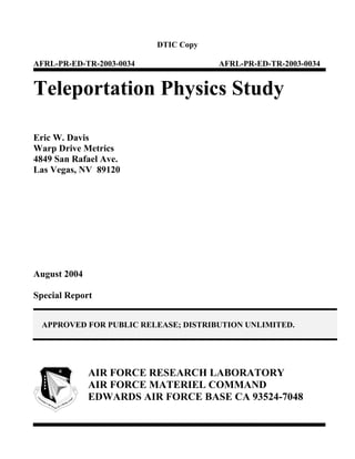
  • 6. List of Figures Figure Page Figure 1. Diagram of a Simultaneous View of Two Remote Compact Regions (Ω1 and Ω2) of Minkowski Space Used to Create the Wormhole Throat ∂Ω, Where Time is Suppressed in This Representation……………..……………………….……………………………………5 Figure 2. The Same Diagram as in Figure 1 Except as Viewed by an Observer Sitting in Region Ω1 Who Looks Through the Wormhole Throat ∂Ω and Sees Remote Region Ω2 (Dotted Area Inside the Circle) on the Other Side………………………………………………………. 6 Figure 3. A Thin Shell of (Localized) Matter-Energy, or Rather the Two-Dimensional Spacelike Hypersurface ∂Ω (via (2.3)), Possessing the Two Principal Radii of Curvature ρ1 and ρ2….…..8 Figure 4. A Schematic of Vacuum Quantum Field Fluctuations (a.k.a. Vacuum Zero Point Field Fluctuations) Involved in the “Light-by-Light” Scattering Process That Affects the Speed of Light…………………………………………………………………………………………13 Figure 5. A Schematic of the Casimir Effect Cavity/Waveguide………………………………………...15 Figure 6. Classical Facsimile Transmission (Modified IBM Press Image)………………………………35 Figure 7. Quantum Teleportation (Modified IBM Press Image)…………………………………………36 Figure 8. Quantum Teleportation (From www.aip.org)..............................................................................43 Approved for public release; distribution unlimited. iv
  • 7. List of Tables Table Page Table 1. Metric Effects in the PV-GR Model When K > 1 (Compared With Reference Frames at Asymptotic Infinity Where K = 1)…………………………………………………………...…21 Table 2. Metric Effects in the PV-GR Model When K < 1 (Compared With Reference Frames at Asymptotic Infinity Where K = 1)……………………………………………………………...22 Table 3. Substantial Gravitational Squeezing Occurs When λ ≥ 8πrs (For Electromagnetic ZPF)............28 Approved for public release; distribution unlimited. v
  • 8. Glossary AEC Average Energy Condition AFRL Air Force Research Laboratory AU Astronomical Unit BBO Beta (β)-Barium Borate CGS Centimeter-Gram-Second CIA Central Intelligence Agency DARPA Defense Advanced Research Projects Agency DEC Dominant Energy Condition DIA Defense Intelligence Agency DNA Deoxyribo Nucleic Acid DoD Department of Defense EPR Einstein, Podolsky and Rosen ESP Extrasensory Perception eV Electron Volt FRW Friedmann-Robertson-Walker FTL Faster-Than-Light IBM International Business Machines INSCOM Intelligence and Security Command IR Infrared MeV Mega-Electron Volt MKS Meter-Kilogram-Second NEC Null Energy Condition NLP Neuro-Linguistic Programming NMR Nuclear Magnetic Resonance NSA National Security Agency PK Psychokinesis PPN Parameterized Post-Newtonian PRC Peoples Republic of China PV-GR Polarizable-Vacuum Representation of General Relativity QED Quantum Electrodynamics QISP Quantum Information Science Program R&D Research and Development SAIC Science Applications International Corporation SEC Strong Energy Condition SRI Stanford Research Institute USSR Union of Soviet Socialist Republics UV Ultraviolet WEC Weak Energy Condition ZPE Zero-Point Energy ZPF Zero-Point Fluctuations Approved for public release; distribution unlimited. vi
  • 9. Acknowledgements This study would not have been possible without the very generous support of Dr. Frank Mead, Senior Scientist at the Advanced Concepts Office of the U.S. Air Force Research Laboratory (AFRL) Propulsion Directorate at Edwards AFB, CA. Dr. Mead’s collegial collaboration, ready assistance, and constant encouragement were invaluable to me. Dr. Mead’s professionalism and excellent rapport with “out-of-the-box” thinkers excites and motivates serious exploration into advanced concepts that push the envelope of knowledge and discovery. The author owes a very large debt of gratitude and appreciation to both Dr. David Campbell, Program Manager, ERC, Inc. at AFRL, Edwards AFB, CA, and the ERC, Inc. staff, for supporting the project contract and for making all the paperwork fuss totally painless. Dr. Campbell and his staff provided timely assistance when the author needed it, which helped make this contract project run smoothly. There are two colleagues who provided important contributions to this study that I wish to acknowledge. First, I would like to express my sincere thanks and deepest appreciation to my first longtime mentor and role model, the late Dr. Robert L. Forward. Bob Forward was the first to influence my interests in interstellar flight and advanced breakthrough physics concepts (i.e., “Future Magic”) when I first met him at an AIAA Joint Propulsion Conference in Las Vegas while I was in high school (ca. 1978). The direction I took in life from that point forward followed the trail of exploration and discovery that was blazed by Bob. I will miss him, but I will never forget him. Second, I would like to express my sincere thanks and appreciation to my longtime friend, colleague and present mentor, Dr. Hal Puthoff, Institute for Advanced Studies-Austin, for our many discussions on applying his Polarizable Vacuum- General Relativity model to a quasi-classical teleportation concept. Hal taught me to expand my mind, and he encourages me to think outside the box. He also gave me a great deal of valuable insight and personal knowledge about the Remote Viewing Program. Last, I would like to offer my debt of gratitude and thanks to my business manager (and spouse), Lindsay K. Davis, for all the hard work she does to make the business end of Warp Drive Metrics run smoothly. Eric W. Davis, Ph.D., FBIS Warp Drive Metrics Las Vegas, NV Approved for public release; distribution unlimited. vii
  • 10. Preface The Teleportation Physics Study is divided into four phases. Phase I is a review and documentation of quantum teleportation, its theoretical basis, technological development, and its potential application. Phase II developed a textbook description of teleportation as it occurs in classical physics, explored its theoretical and experimental status, and projected its potential applications. Phase III consisted of a search for teleportation phenomena occurring naturally or under laboratory conditions that can be assembled into a model describing the conditions required to accomplish the disembodied conveyance of objects. The characteristics of teleportation were defined, and physical theories were evaluated in terms of their ability to completely describe the phenomenon. Presently accepted physics theories, as well as theories that challenge the current physics paradigm were investigated for completeness. The theories that provide the best chance of explaining teleportation were selected, and experiments with a high chance of accomplishing teleportation were identified. Phase IV is the final report. The report contains five chapters. Chapter 1 is an overview of the textbook descriptions for the various teleportation phenomena that are found in nature, in theoretical physics concepts, and in experimental laboratory work. Chapter 2 proposes two quasi-classical physics concepts for teleportation: the first is based on engineering the spacetime metric to induce a traversable wormhole; the second is based on the polarizable-vacuum-general relativity approach that treats spacetime metric changes in terms of equivalent changes in the vacuum permittivity and permeability constants. These concepts are theoretically developed and presented. Promising laboratory experiments were identified and recommended for further research. Chapter 3 presents the current state-of-art of quantum teleportation physics, its theoretical basis, technological development, and its applications. Key theoretical, experimental, and applications breakthroughs were identified, and a series of theoretical and experimental research programs are proposed to solve technical problems and advance quantum teleportation physics. Chapter 4 gives an overview of alternative teleportation concepts that challenge the present physics paradigm. These concepts are based on the existence of parallel universes/spaces and/or extra space dimensions. The theoretical and experimental work that has been done to develop these concepts is reviewed, and a recommendation for further research is made. Last, Chapter 5 gives an in-depth overview of unusual teleportation phenomena that occur naturally and under laboratory conditions. The teleportation phenomenon discussed in the chapter is based on psychokinesis (PK), which is a category of psychotronics. The U.S. military-intelligence literature is reviewed, which relates the historical scientific research performed on PK-teleportation in the U.S., China and the former Soviet Union. The material discussed in the chapter largely challenges the current physics paradigm; however, extensive controlled and repeatable laboratory data exists to suggest that PK-teleportation is quite real and that it is controllable. The report ends with a combined list of references. Approved for public release; distribution unlimited. viii
  • 11. 1.0 INTRODUCTION 1.1 Introduction The concept of teleportation was originally developed during the Golden Age of 20th century science fiction literature by writers in need of a form of instantaneous disembodied transportation technology to support the plots of their stories. Teleportation has appeared in such SciFi literature classics as Algis Budry’s Rogue Moon (Gold Medal Books, 1960), A. E. van Vogt’s World of Null-A (Astounding Science Fiction, August 1945), and George Langelaan’s The Fly (Playboy Magazine, June 1957). The Playboy Magazine short story led to a cottage industry of popular films decrying the horrors of scientific technology that exceeded mankind’s wisdom: The Fly (1958), Return of the Fly (1959), Curse of the Fly (1965), The Fly (a 1986 remake), and The Fly II (1989). The teleportation concept has also appeared in episodes of popular television SciFi anthology series such as The Twilight Zone and The Outer Limits. But the most widely recognized pop-culture awareness of the teleportation concept began with the numerous Star Trek television and theatrical movie series of the past 39 years (beginning in 1964 with the first TV series pilot episode, The Cage), which are now an international entertainment and product franchise that was originally spawned by the late genius television writer-producer Gene Roddenberry. Because of Star Trek everyone in the world is familiar with the “transporter” device, which is used to teleport personnel and material from starship to starship or from ship to planet and vice versa at the speed of light. People or inanimate objects would be positioned on the transporter pad and become completely disintegrated by a beam with their atoms being patterned in a computer buffer and later converted into a beam that is directed toward the destination, and then reintegrated back into their original form (all without error!). “Beam me up, Scotty” is a familiar automobile bumper sticker or cry of exasperation that were popularly adopted from the series. However, the late Dr. Robert L. Forward (2001) stated that modern hard-core SciFi literature, with the exception of the ongoing Star Trek franchise, has abandoned using the teleportation concept because writers believe that it has more to do with the realms of parapsychology/paranormal (a.k.a. psychic) and imaginative fantasy than with any realm of science. Beginning in the 1980s developments in quantum theory and general relativity physics have succeeded in pushing the envelope in exploring the reality of teleportation. A crescendo of scientific and popular literature appearing in the 1990s and as recently as 2003 has raised public awareness of the new technological possibilities offered by teleportation. As for the psychic aspect of teleportation, it became known to Dr. Forward and myself, along with several colleagues both inside and outside of government, that anomalous teleportation has been scientifically investigated and separately documented by the Department of Defense. It has been recognized that extending the present research in quantum teleportation and developing alternative forms of teleportation physics would have a high payoff impact on communications and transportation technologies in the civilian and military sectors. It is the purpose of this study to explore the physics of teleportation and delineate its characteristics and performances, and to make recommendations for further studies in support of Air Force Advanced Concepts programs. 1.2 The Definitions of Teleportation Before proceeding, it is necessary to give a definition for each of the teleportation concepts I have identified during the course of this study: Approved for public release; distribution unlimited. 1
  • 12. Teleportation – SciFi: the disembodied transport of persons or inanimate objects across space by advanced (futuristic) technological means (adapted from Vaidman, 2001). We will call this sf- Teleportation, which will not be considered further in this study. Teleportation – psychic: the conveyance of persons or inanimate objects by psychic means. We will call this p-Teleportation. Teleportation – engineering the vacuum or spacetime metric: the conveyance of persons or inanimate objects across space by altering the properties of the spacetime vacuum, or by altering the spacetime metric (geometry). We will call this vm-Teleportation. Teleportation – quantum entanglement: the disembodied transport of the quantum state of a system and its correlations across space to another system, where system refers to any single or collective particles of matter or energy such as baryons (protons, neutrons, etc.), leptons (electrons, etc.), photons, atoms, ions, etc. We will call this q-Teleportation. Teleportation – exotic: the conveyance of persons or inanimate objects by transport through extra space dimensions or parallel universes. We will call this e-Teleportation. We will examine each of these in detail in the following chapters and determine whether any of the above teleportation concepts encompass the instantaneous and or disembodied conveyance of objects through space. Approved for public release; distribution unlimited. 2
  • 13. 2.0 vm-TELEPORTATION 2.1 Engineering the Spacetime Metric A comprehensive literature search for vm-Teleportation within the genre of spacetime metric engineering yielded no results. No one in the general relativity community has thought to apply the Einstein field equation to determine whether there are solutions compatible with the concept of teleportation. Therefore, I will offer two solutions that I believe will satisfy the definition of vm- Teleportation. The first solution can be found from the class of traversable wormholes giving rise to what I call a true “stargate.” A stargate is essentially a wormhole with a flat-face shape for the throat as opposed to the spherical-shaped throat of the Morris and Thorne (1988) traversable wormhole, which was derived from a spherically symmetric Lorentzian spacetime metric that prescribes the wormhole geometry (see also, Visser, 1995 for a complete review of traversable Lorentzian wormholes): ds 2 = −e 2φ ( r ) c 2 dt 2 + [1 − b(r ) r ]−1 dr 2 + r 2 d Ω 2 (2.1), where by inspection we can write the traversable wormhole metric tensor in the form  − e 2φ ( r ) 0 0 0    0 [1 − b(r ) r ]−1 0 0 gαβ =  (2.2)  0 0 r2 0    0   0 0 r 2 sin 2 θ   using standard spherical coordinates, where c is the speed of light, α,β ≡ (0 = t, 1 = r, 2 = θ, 3 = ϕ) are the time and space coordinate indices (-∞ < t < ∞; r: 2πr = circumference; 0 ≤ θ ≤ π; 0 ≤ ϕ ≤ 2π), dΩ2 = dθ2 + sin2θdϕ2, φ(r) is the freely specifiable redshift function that defines the proper time lapse through the wormhole throat, and b(r) is the freely specifiable shape function that defines the wormhole throat’s spatial (hypersurface) geometry. Such spacetimes are asymptotically flat. The Einstein field equation requires that a localized source of matter-energy be specified in order to determine the geometry that the source induces on the local spacetime. We can also work the Einstein equation backwards by specifying the local geometry in advance and then calculate the matter-energy source required to induce the desired geometry. The Einstein field equation thus relates the spacetime geometry terms comprised of the components of the metric tensor and their derivatives (a.k.a. the Einstein tensor) to the local matter- energy source terms comprised of the energy and stress-tension densities (a.k.a. the stress-energy tensor). The flat-face wormhole or stargate is derived in the following section. 2.1.1 Wormhole Thin Shell Formalism The flat-face traversable wormhole solution is derived from the thin shell (a.k.a. junction condition or surface layer) formalism of the Einstein equations (Visser, 1989; see also, Misner, Thorne and Wheeler, 1973). We adapt Visser’s (1989) development in the following discussion. The procedure is to take two copies of flat Minkowski space and remove from each identical regions of the form Ω × ℜ, where Ω is a three-dimensional compact spacelike hypersurface and ℜ is a timelike straight line (time axis). Then identify these two incomplete spacetimes along the timelike boundaries ∂Ω × ℜ. The resulting spacetime Approved for public release; distribution unlimited. 3
  • 14. is geodesically complete and possesses two asymptotically flat regions connected by a wormhole. The throat of the wormhole is just the junction ∂Ω (a two-dimensional space-like hypersurface) at which the two original Minkowski spaces are identified (see Figures 1 and 2). Approved for public release; distribution unlimited. 4
  • 15. Figure 1. Diagram of a Simultaneous View of Two Remote Compact Regions (Ω1 and Ω2) of Minkowski Space Used to Create the Wormhole Throat ∂Ω, Where Time is Suppressed in This Representation (adapted from Bennett et al., 1995) Approved for public release; distribution unlimited. 5
  • 16. Figure 2. The Same Diagram as in Figure 1 Except as Viewed by an Observer Sitting in Region Ω1 Who Looks Through the Wormhole Throat ∂Ω and Sees Remote Region Ω2 (Dotted Area Inside the Circle) on the Other Side Approved for public release; distribution unlimited. 6
  • 17. The resulting spacetime is everywhere Riemann-flat except possibly at the throat. Also, the stress- energy tensor in this spacetime is concentrated at the throat with a δ-function singularity there. This is a consequence of the fact that the spacetime metric at the throat is continuous but not differentiable, while the connection is discontinuous; thus causing the Riemann curvature to possess a δ-function singularity (causing undesirable gravitational tidal forces) there. The magnitude of this δ-function singularity can be calculated in terms of the second fundamental form on both sides of the throat, which we presume to be generated by a localized thin shell of matter-energy. The second fundamental form represents the extrinsic curvature of the ∂Ω hypersurface (i.e., the wormhole throat), telling how it is curved with respect to the enveloping four-dimensional spacetime. The form of the geometry is simple, so the second fundamental form at the throat is calculated to be (McConnell, 1957): κ 0 0 0   K i ± j = ±  0 κ1 0 0 0 κ2    (2.3), 0 0 0    = ±  0 1 ρ1 0  0 0 1 ρ2    where i,j = 0,1,2 and Kij± is the second fundamental form. The full 4×4 matrix Kαβ has been reduced to 3×3 form, as above, for computational convenience because the thin shell (or hypersurface) is essentially a two-surface embedded in three-space. The overall ± sign in equation (2.3) comes from the fact that a unit normal points outward from one side of the surface and points inward on the other side. We hereafter drop the ± sign for the sake of brevity in notation. The quantities κ0, κ1, and κ2 measure the extrinsic curvature of the thin shell of local matter-energy (i.e., the stuff that induces the wormhole throat geometry). Since the wormhole throat is a space-like hypersurface, we can exclude time-like hypersurfaces and their components in the calculations. Therefore we set κ0 = 0 in equation (2.3) because it is the time-like extrinsic curvature for the time-like hypersurface of the thin shell of matter-energy. As seen in equation (2.3) κ1 and κ2 are simply related to the two principal radii of curvature ρ1 and ρ2 (defined to be the eigenvalues of Kij) of the two-dimensional spacelike hypersurface ∂Ω (see Figure 3). It should be noted that a convex surface has positive radii of curvature, while a concave surface has negative radii of curvature. Approved for public release; distribution unlimited. 7
  • 18. Figure 3. A Thin Shell of (Localized) Matter-Energy, or Rather the Two-Dimensional Spacelike Hypersurface ∂Ω (via (2.3)), Possessing the Two Principal Radii of Curvature ρ1 and ρ2 Approved for public release; distribution unlimited. 8
  • 19. It is a standard result of the thin shell or junction condition formalism that the Einstein field equation may be cast in terms of the surface stress-energy tensor Sij of the thin matter-energy shell localized in ∂Ω (note: we are exploiting the symmetry of the wormhole with respect to interchange of the two flat regions Ω1 and Ω2): c4 Si j = − 4π G ( K i j − δ i j K k k ) (2.4), where G is Newton’s gravitational constant and δij is the (three-dimensional) unit matrix. Kkk is the trace of equation (2.3): K k k = Tr K i j 1 1 (2.5) = + ρ1 ρ2 and  1 1   + 0 0   ρ1 ρ 2   1 1  δ i j K kk = 0 + 0  (2.6).  ρ1 ρ2   1 1   0  0 +   ρ1 ρ 2   Substituting (2.3) and (2.6) into (2.4) gives (after simplification):  1 1  ρ +ρ 0 0  c4   1 2 S j= i  0 1 ρ2 0  (2.7). 4π G    0 0 1 ρ1      The thin matter-energy shell’s surface stress-energy tensor may be interpreted in terms of the surface energy density σ and principal surface tensions ϑ1 and ϑ2:  −σ 0 0    Si j =  0 −ϑ1 0  (2.8).  0 0 −ϑ2    Thus we arrive at the Einstein field equation by equating (2.8) and (2.7) and multiplying both sides by –1: Approved for public release; distribution unlimited. 9
  • 20.  1 1  ρ +ρ 0 0  σ 0 0 c4   1 2    0 ϑ1 0 =−  0 4π G  1 ρ2 0   (2.9), 0 0 ϑ2  1 ρ1     0 0     which gives the final result c4  1 1  σ =−  +  (2.10a) 4π G  ρ1 ρ 2  c4 1 ϑ1 = − (2.10b) 4π G ρ 2 c4 1 ϑ2 = − (2.10c). 4π G ρ1 These are the Einstein equations. Equations (2.10a-c) imply that (for ∂Ω convex) we are dealing with negative surface energy density and negative surface tensions. This result is in fact the primary matter- energy requirement for traversable wormholes, as was proved by Morris and Thorne (1988), and later by Visser (1995), within the paradigm of classical Einstein general relativity. The negative surface tension (= positive outward pressure, a.k.a. gravitational repulsion or antigravity) is needed to keep the throat open and stable against collapse. The reader should not be alarmed at this result. Negative energies and negative stress-tensions are an acceptable result both mathematically and physically, and they manifest gravitational repulsion (antigravity!) in and around the wormhole throat. One only needs to understand what it means for stress-energy to be negative within the proper context. In general relativity the term “exotic” is used in place of “negative.” The effects of negative energy have been produced in the laboratory (the Casimir Effect is one example). In short, negative energy arises from Heisenberg’s quantum uncertainty principle, which requires that the energy density of any electromagnetic, magnetic, electric or other fields must fluctuate randomly. Even in a vacuum, where the average energy density is zero, the energy density fluctuates. This means that the quantum vacuum can never remain truly empty in the classical sense of the term. The quantum picture of the vacuum is that of a turbulent plenum of virtual (i.e., energy non-conserving) particle pairs that spontaneously pop in and out of existence. The notion of “zero energy” in quantum theory corresponds to the vacuum being filled with such fluctuations going on. This issue is further elaborated on and clarified in greater detail in Appendix A. We will also revisit this in Section 2.2. Finally, it should be noted that for the analysis in this section we assumed an ultrastatic wormhole [i.e., g00 ≡ 1 ⇒ φ(r) = 0 in equation (2.1)] with the “exotic” matter-energy confined to a thin layer, and we dispensed with the assumption of spherical symmetry. We can now build a wormhole-stargate and affect vm-Teleportation such that a traveler stepping into the throat encounters no exotic matter-energy there. This will require that our wormhole be flat shaped. To make the wormhole flat requires that we choose the throat ∂Ω to have at least one flat face (picture the thin shell in Figure 3 becoming a flat shell). On that face the two principal radii of curvature become ρ1 = ρ2 = ∞ as required by standard geometry. Substituting this into equations (2.10a-c) gives σ = ϑ1 = ϑ2 = 0 (2.11), Approved for public release; distribution unlimited. 10
  • 21. which is a remarkable result. A further consequence of this is that now Kij = 0, thus making the Riemann curvature and stress-energy tensors (Riemann: Rαβ ~ Kαβ; stress-energy: Tαβ ~ Kαβ) at the throat become zero such that the associated δ-function singularities disappear there. This means that a traveler encountering and going through such a wormhole will feel no tidal gravitational forces and see no exotic matter-energy (that threads the throat). A traveler stepping through the throat will simply be teleported into the other remote spacetime region or another universe (note: the Einstein equation does not fix the spacetime topology, so it is possible that wormholes are inter-universe as well as intra-universe tunnels). We construct such a teleportation stargate by generating a thin shell or surface layer of “exotic” matter- energy much like a thin film of soap stretched across a loop of wire. 2.1.2 “Exotic” Matter-Energy Requirements Now we have to estimate the amount of negative (or exotic) mass-energy that will be needed to generate and hold open a vm-Teleportation wormhole. A simple formula originally due to Visser (1995) for short-throat wormholes using the thin shell formalism gives: rthroat c 2 M wh =− G rthroat = −(1.3469 x1027 kg ) (2.12), 1 meter r = −(0.709 M Jupiter ) throat 1 meter where Mwh is the mass required to build the wormhole, rthroat is a suitable measure of the linear dimension (radius) of the throat, and MJupiter is the mass of the planet Jupiter (1.90×1027 kg). Equation (2.12) demonstrates that a mass of –0.709 MJupiter (or –1.3469×1027 kg) will be required to build a wormhole 1 meter in size. As the wormhole size increases the mass requirement grows negative-large, and vice versa as the wormhole size decreases. After being alarmed by the magnitude of this, one should note that Mwh is not the total mass of the wormhole as seen by observers at remote distances. The non-linearity of the Einstein field equations dictates that the total mass is zero (actually, the total net mass being positive, negative or zero in the Newtonian approximation depending on the details of the negative energy configuration constituting the wormhole system). And finally, Visser et al. (2003) have demonstrated the existence of spacetime geometries containing traversable wormholes that are supported by arbitrarily small quantities of exotic matter-energy, and they proved that this was a general result. In Section 2.3 we will discuss how or whether we can create such a wormhole in the laboratory. 2.2 Engineering the Vacuum Engineering the spacetime vacuum provides a second solution that also satisfies the definition of vm- Teleportation. The concept of “engineering the vacuum” was first introduced to the physics community by Lee (1988). Lee stated: “The experimental method to alter the properties of the vacuum may be called vacuum engineering…If indeed we are able to alter the vacuum, then we may encounter some new phenomena, totally unexpected.” This new concept is based on the now-accepted fact that the vacuum is characterized by physical parameters and structure that constitutes an energetic medium which pervades the entire extent of the Approved for public release; distribution unlimited. 11
  • 22. universe. We note here the two most important defining properties of the vacuum in this regard (Puthoff et al., 2002): Within the context of quantum field theory the vacuum is the seat of all energetic particle and field fluctuations. Within the context of general relativity theory the vacuum is the seat of a spacetime structure (or metric) that encodes the distribution of matter and energy. We begin our look into this concept by examining the propagation of light through space. We know from quantum field theory that light propagating through space interacts with the vacuum quantum fields (a.k.a. vacuum quantum field fluctuations). The observable properties of light, including the speed of light, are determined by these interactions. Vacuum quantum interactions with light lead to an effect on the speed of light that is due to the absorption of photons (by the vacuum) to form virtual electron- positron pairs followed by the quick re-emission (from the vacuum) of the photon (see Figure 4). The virtual particle pairs are very short lived because of the large mismatch between the energy of a photon and the rest mass-energy of the particle pair. A key point is that this process makes a contribution to the observed vacuum permittivity ε0 (and permeability µ0) constant and, therefore, to the speed of light c [c = (ε0µ0)−1/2]. Approved for public release; distribution unlimited. 12
  • 23. Figure 4. A Schematic of Vacuum Quantum Field Fluctuations (a.k.a. Vacuum Zero Point Field Fluctuations) Involved in the “Light-by-Light” Scattering Process That Affects the Speed of Light (from Chown, 1990) Approved for public release; distribution unlimited. 13
  • 24. The role of virtual particle pairs in determining the ε0 (µ0) of the vacuum is analogous to that of atoms/molecules in determining the relative permittivity ε (and µ) of a dielectric material. We know that the absorption/re-emission of photons by atoms/molecules in a transparent medium (note: there are no strongly absorbing resonances, so the atoms/molecules remain in their excited states for a very short time before re-emitting photons) is responsible for the refractive index of the medium, which results in the reduction of the speed of light for photons propagating through the medium. This absorption/re-emission process is also known in physics as a scattering process. We know from experiment that a change in the medium leads to a change in ε (µ), thus resulting in a change of the refractive index. The key point arising from this analogy is that a modification of the vacuum produces a change in ε0 (µ0) resulting in a subsequent change in c, and hence, a corresponding change in the vacuum refraction index. Scharnhorst (1990) and Latorre et al. (1995) have since proved that the suppression of light scattering by virtual particle pairs (a.k.a. coherent light-by-light scattering) in the vacuum causes an increase in the speed of light accompanied by a decrease in the vacuum refraction index. This very unique effect is accomplished in a Casimir Effect capacitor cavity (or waveguide) whereby the vacuum quantum field fluctuations (a.k.a. zero-point fluctuations or ZPF) inside have been modified (becoming anisotropic and non-translational invariant) to satisfy the electromagnetic boundary conditions imposed by the presence of the capacitor plates (or waveguide walls). The principal result of this modification is the removal of the electromagnetic zero-point energy (ZPE) due to the suppression of vacuum ZPE modes with wavelengths longer than the cavity/waveguide cutoff (λ0 = 2d, where d = plate separation; see Figure 5). This removal of free space vacuum ZPE modes suppresses the scattering of light by virtual particle pairs, thus producing the speed of light increase (and corresponding decrease in the vacuum refraction index). We know from standard optical physics and quantum electrodynamics (QED) that the optical phase and group velocities can exceed c under certain physical conditions, but dispersion always ensures that the signal velocity is ≤ c. But recent QED calculations (see, Scharnhorst, 1990 and Latorre et al., 1995) have proved that in the Casimir Effect system, the dispersive effects are much weaker still than those associated with the increase in c so that the phase, group and signal velocities will therefore all increase by the same amount. Note that, in general, no dispersion shows up in all of the modified vacuum effects examined by investigators. Approved for public release; distribution unlimited. 14
  • 25. Figure 5. A Schematic of the Casimir Effect Cavity/Waveguide (from Chown, 1990) Approved for public release; distribution unlimited. 15
  • 26. Examples demonstrating the increase in light speed (decrease in vacuum refraction index) via the Casimir Effect vacuum and other modified vacuum effects, as well as those effects producing a decrease in light speed (increase in vacuum refraction index), are described as follows. The vacuum modification effect on the speed of light described in the previous paragraph is (Scharnhorst, 1990): c⊥∗  11 e4  = 1 + 6  ( = c0 = ε 0 = µ0 = 1) c0  2 i(45) 2 (me a) 4  (2.13),  11π 2 2 1  = 1 + α 4  >1  8100 (me a )  where c⊥* is the (modified) speed of light propagation perpendicular to the Casimir Effect capacitor plates, c0 is the speed of light in free space (3×10⁸ m/s in MKS units), me is the electron mass, α is the fine structure constant (≈ 1/137), e is the electron charge (e2 = 4πα in quantum field theory natural units), a is the plate separation, ħ is Planck’s reduced constant, and ε0 is the vacuum permittivity constant. The condition ħ = c0 = ε0 = µ0 = 1 stresses that (2.13), and all the equations that follow, are in quantum field theory natural units. The speed of light and vacuum refraction index measured parallel to the plates is unchanged from their free space values (c|| = c0, n|| = n0 = 1). The modified vacuum refraction index measured perpendicular to the plates is (Scharnhorst, 1990):  11 e4  n⊥ =  1 − 6 2 4  <1 ( = c0 = ε 0 = µ 0 = 1) (2.14).  2 i(45) (me a )  Equations (2.13) and (2.14) show that in general n⊥ < 1 and c⊥* > c0. But c⊥* → c0 and n⊥ → 1 when a → ∞ as expected, since we are now allowing all of the vacuum ZPE modes to re-enter the Casimir cavity in this case. We now survey the additional examples of modified vacuums which increase/decrease light speed (from Latorre et al., 1995): For light (photons) propagating in a Friedmann-Robertson-Walker (FRW) vacuum (i.e., a homogeneous and isotropic Robertson-Walker gravitational background with Friedmann cosmology): c∗  11 ρ + p = 1 + α G r 2  > 1 ( = c0 = ε 0 = µ 0 = 1) (2.15), c0  45 me  where c* is the modified vacuum speed of light, G is Newton’s constant, ρr is the energy density and p is the pressure of a radiation-dominated universe (p = ρr/3). Here the speed of light is increased. For light (photons) propagating in a homogeneous and isotropic thermal vacuum: c∗  44π 2 2 T 4  = 1 − α  <1 ( = c0 = ε 0 = µ 0 = k B = 1) (2.16), c0  2025 me 4  Approved for public release; distribution unlimited. 16
  • 27. where T is the temperature of the vacuum and kB is the Boltzmann constant. Here the speed of light is decreased. For light (photons) propagating in an anisotropic vacuum given by an external constant uniform magnetic field B: c∗  8 B2  = 1 − α 2 4 sin 2 θ  < 1 ( = c0 = ε 0 = µ0 = 1) c0  45 me  (2.17), c⊥  14 2 B ∗ 2  = 1 − α sin 2 θ  < 1 c0  45 me 4  where the speed of light is decreased in this vacuum for polarizations coplanar (||) with and perpendicular (⊥) to the plane defined by B and the direction of propagation, and θ is the angle between B and the direction of propagation. Latorre et al. (1995) calculated the polarization-average of (2.17) to give the averaged (modified) speed of light in the B-field: c∗  22 2 B 2  = 1 − α  <1 ( = c0 = ε 0 = µ 0 = 1) (2.18). c0  135 me 4  For light (photons) propagating in an anisotropic vacuum given by an external constant uniform electric field E, the polarization-averaged modified speed of light is: c∗  22 2 E2  = 1 − α  <1 ( = c0 = ε 0 = µ 0 = 1) (2.19). c0  135 me 4  Here the speed of light is decreased. Equations (2.16) – (2.19) are the result of vacuum modifications that populate the vacuum with virtual or real particles that induce coherent (light-by-light) scattering, which reduces the speed of massless particles. By examining the form of equations (2.13) and (2.15) – (2.19) Latorre et al. (1995) discovered that the low energy modification of the speed of light is proportional to the ratio of the modified vacuum energy density (as compared to the standard vacuum energy density, ρvac = 0) over me4, with a universal numerical coefficient and the corresponding coupling constants. And a general rule became apparent from their analysis that is applicable to modified vacua for massive and massless quantum field theories, for low energy: c* > c0 (vacuum refraction index < 1) when the modified vacuum has a lower energy density c* < c0 (vacuum refraction index > 1) when the modified vacuum has a higher energy density c* = c0 (vacuum refraction index = 1) when the vacuum is free (or un-modified) with ρvac = 0 The first two rules explain the sign of the change of the speed of light. From this rule and the mathematical commonality between the form of (2.13) and (2.15) – (2.19) Latorre et al. (1995) found a single unifying expression to replace these equations: c∗ 44 2 ρ = 1− α ( = c0 = ε 0 = µ0 = 1) (2.20), c0 135 me 4 Approved for public release; distribution unlimited. 17
  • 28. where ρ is the energy density of the modified vacua under consideration such that ρ → ρE ~ E2 for the electric field vacuum, ρ → ρB ~ B2 for the magnetic field vacuum, and ρ → ρT ~ π2T4 for the thermal vacuum. If the vacuum is a FRW gravitational vacuum, then one has to substitute one factor of α in (2.20) by −me2G and ρ → ρr. Equation (2.13) for the Casimir Effect vacuum studied earlier is recovered when ρ → ρCasimir = −(π2/240)a−4. Let us recast (2.20) into a more useful form. We subtract one from both sides of (2.20), do some algebra, and thus define the ratio of the change in the speed of light ∆c in a modified vacuum to the speed of light in free space c0: c∗ c∗ − c0 ∆c −1 = ≡ c0 c0 c0 ∆c 44 2 ρ =− α ( = c0 = ε 0 = µ0 = 1) (2.21). c0 135 me 4 Equations (2.20) and (2.21) are in quantum field theory natural units, which is completely undesirable for estimating physically measurable values of ∆c/c0. We thus transform or “unwrap” (2.20) and (2.21) back into MKS or CGS units by making the following substitutions (Puthoff, 2003) ρ ρ (natural units) → (MKS or CGS units) c mc me (natural units) → e (MKS or CGS units) , and after some algebra and rearranging we arrive at the final result: 3 c∗ 44 2 ρ   = 1− α 2   (2.22) c0 135 me c0  me c0  and 3 ∆c 44 2 ρ   =− α 2   (2.23), c0 135 me c0  me c0  where all quantities are now in MKS or CGS units. We chose the former units so that c0 = 3×10⁸ m/s, ħ = 1.055×10⁻³⁴ J-s, me = 9.11×10⁻³¹ kg, and α = 1/137. Note that the ratio of the modified vacuum energy density to the electron rest-mass energy has the dimension of (volume)−1 while the quantity in the bracket is the cubed Compton wavelength of the electron having the dimension of (volume), and the product of these is dimensionless. An excellent example for estimating the magnitude of the change in the speed of light (in a modified vacuum) is the Casimir Effect vacuum, since Casimir Effect experiments are common and widespread such that this would be ideal to experimentally test (2.23). We substitute the Casimir vacuum energy density ρCasimir = −(π2ħc0/240)a−4 (in MKS units) into (2.23), do the algebra, insert the MKS values for the physical constants, and make further simplifications to get: Approved for public release; distribution unlimited. 18
  • 29. 3 ∆c 44 2  π 2 c0  1   =− α − 4  2   c0 135  240 a  me c0  me c0  4 11 2 2   = απ   (2.24), 8100  me c0 a  ≈ (1.59 × 10−56 ) a −4 where a (the plate separation) is in meters. Another useful equation is:  ∆c  c∗ = 1 +  c0 (2.25),  c0  where we make the substitution c* → c⊥* for the present case. H. E. Puthoff and the author (Puthoff, 2003) compared the third line in (2.24) with equation (26) in Scharnhorst (1990) and discovered that the result cited there is in error, because the numerical coefficient is four orders of magnitude too small (Scharnhorst originally pointed out this error to Forward, 1996). We now set a = 10−6 m (1 µm) and we get ∆c/c0 ≈ 10−32 and c⊥* ≈ c0, which is a horrifically small 1 part in 1032 change that we cannot hope to measure at present. But for a = 10−10 m (1 Å) we get ∆c/c0 ≈ 10−16 and c⊥* ≈ c0, which is a 1 part in 1016 change that could be measurable at present or in the very near future using high precision laser technology. Last, for a = 1.1229×10⁻¹⁴ m (11.229 fm or ≈ 11 times the nuclear diameter; 1 fm = 10−15 m) we find that ∆c/c0 ≈ 1 and c⊥* ≈ 2c0. We are not able to do technical work at nuclear distances at this time; however, that could change as ultrahigh precision measurement technology continues to evolve. The threshold for the onset of significant changes in light speed occurs when a < 10−12 m. This result is generally true for the other modified vacua surveyed in (2.15) – (2.19), since accessible (everyday) values for electric and magnetic field strengths, thermal temperatures and radiation densities are not large enough to overcome the size of the electron mass to create a measurable effect. However, there is a class of ultrahigh intensity tabletop lasers that have achieved such extreme electric and magnetic field strengths and temperatures that it may now be possible to consider using them to explore vacuum modification effects in the lab. We will return to this theme in a later section. •Key Point: As disappointing as the Casimir Effect vacuum (and other modified vacua) results are, it should be strongly pointed out that special relativity theory says that if in one inertial reference frame an object travels only one part in 1016 (or even one part in 1032) times faster than c0, then one can find another reference frame where departure and arrival times of the object are simultaneous, and thus the velocity is infinite. This is what motivates us to look at a teleportation mechanism based on engineering of the vacuum. •Technical Notes: Equation (2.15) is interpreted as an increase in the speed of light due to a decrease in the number of vacuum ZPE modes. However, this effect is totally unrelated to light-by-light scattering in the vacuum because the gravitational background “squeezes” (as in squeezed quantum optics states; see Davis, 1999a) the ZPE modes, therefore reducing the vacuum energy density. We further note that the coefficient of 11 is the same for the gravitational vacuum as for the other modified vacua examples based on QED. This factor also appears in the coefficient of the Euler-Poincare characteristic spin-½ contribution to the gravitational trace anomaly (Birrell and Davies, 1982). It is beyond the scope of this study to consider the deep connections between quantum field theory and gravitation. Approved for public release; distribution unlimited. 19
  • 30. We have excluded from our survey the Latorre et al. (1995) results pertaining to all other (high or low energy) modifications of the speed of massless particles. That is because the other examples invoked different QED theories possessing massless (me = 0), massive and intrinsic mass scales that introduced complex correction terms (beyond the leading low energy terms surveyed above) which are mass-related or running mass-related, and they introduced no new speed modification effects (beyond the low energy electron-positron virtual pair contributions); or no genuine speed modification was possible (especially for the massless Quantum Chromodynamic sector involving pseudo-Goldstone particles). There is ongoing (very noisy) controversy within the physics community over the effects of c* > c0 on causality. As this topic is beyond the scope of this study, I will make three points in this regard: 1) There are no grounds for microcausality violations in accordance with Drummond and Hathrell (1980). 2) A new definition of causality is in order for FTL (faster- than-light) phenomena. 3) Investigators have found that time machines (a.k.a. closed timelike curves) do not affect Gauss’s theorem, and thus do not affect the derivation of global conservation laws from differential ones (Friedman et al., 1990). The standard conservation laws remain globally valid while retaining a natural quasi-local interpretation for spacetimes possessing time machines (for example, asymptotically flat wormhole spacetimes). Thorne (1993) states that it may turn out that causality is violated at the macroscopic scale. Even if causality is obeyed macroscopically, then quantum gravity might offer finite probability amplitudes for microscopic spacetime histories possessing time machines. Li and Gott (1998) found a self-consistent vacuum for quantum fields in Misner space (a simple flat space with closed timelike curves), for which the renormalized stress-energy tensor is regular (in fact zero) everywhere. This implies that closed timelike curves could exist at least at the level of semi-classical quantum gravity theory. Therefore, FTL causality paradoxes are just a reflection of our ignorance or inadequate comprehension of the physics of chronology and causality. In this section we have shown how “vacuum engineering” can modify the speed of light, and how this can, in principle, lead to vm-Teleportation. The vacuum modification concepts summarized above lead us to a formal theory that implements the concept of vacuum engineering within a framework that parallels general relativity theory. This theory is called the Polarizable-Vacuum Representation of General Relativity. In the next section we will introduce and summarize this theory. 2.2.1 The Polarizable-Vacuum Representation of General Relativity The polarizable-vacuum representation of general relativity (a.k.a. PV-GR) treats the vacuum as a polarizable medium of variable refractive index (Puthoff, 1999a, 2002a, b; Puthoff et al., 2002) exemplifying the concept of the vacuum modification (or vacuum engineering) effects surveyed and discussed in the previous section. The PV-GR approach treats spacetime metric changes in terms of equivalent changes in the vacuum permittivity and permeability constants (ε0 and µ0), essentially along the lines of the “THεµ” methodology (see Appendix B for a brief description of this) used in comparative studies of alternative metric theories of gravity (Lightman and Lee, 1973; Will, 1974, 1989, 1993; Haugan and Will, 1977). Such an approach, relying as it does on parameters familiar to engineers, can be considered a “metric engineering” approach. Maxwell's equations in curved space are treated in the isomorphism of a polarizable medium of variable refractive index in flat space (Volkov et al., 1971); the bending of a light ray near a massive body is modeled as due to an induced spatial variation in the refractive index of the vacuum near the body; the reduction in the velocity of light in a gravitational potential is represented by an effective increase in the refractive index of the vacuum, and so forth. This optical-engineering approach has been shown to be quite general (de Felice, 1971; Evans et al., 1996a, b). Approved for public release; distribution unlimited. 20
  • 31. As recently elaborated by Puthoff (1999a, 2002a, b; Puthoff et al., 2002) the PV-GR approach, which was first introduced by Wilson (1921) and then developed by Dicke (1957, 1961), can be carried out in a self-consistent way so as to reproduce to appropriate order both the equations of general relativity and the match to the standard astrophysics weak-field experimental (PPN parameters and other) tests of those equations while posing testable modifications for strong-field conditions. It is in application that the PV- GR approach demonstrates its intuitive appeal and provides additional insight into what is meant by a curved spacetime metric. Specifically, the PV-GR approach treats such measures as the speed of light, the length of rulers (atomic bond lengths), the frequency of clocks, particle masses, and so forth, in terms of a variable vacuum dielectric constant K in which the vacuum permittivity ε0 transforms as ε0 → Kε0 and the vacuum permeability transforms as µ0 → Kµ0 (see also, Rucker, 1977). In a planetary or solar gravitational potential K = exp(2GM/rc02) > 1 (M is a local mass distribution, r is the radial distance from the center of M) while K = 1 in “empty” or free asymptotic space (Puthoff, 1999a, 2002a, b; Puthoff et al., 2002). In the former case, the speed of light is reduced, light emitted from an atom is redshifted as compared with a remote static atom (where K = 1), clocks run slower, objects/rulers shrink, etc. See Table 1. Table 1. Metric Effects in the PV-GR Model When K > 1 (Compared With Reference Frames at Asymptotic Infinity Where K = 1; adapted from Puthoff et al., 2002) Variable Determining Equation K>1 (subscript 0 is asymptotic value (typical mass distribution, M) where K = 1) modified speed of light c*(K) c* = c0/K speed of light < c0 Modified mass m(K) m = m0K3/2 effective mass increases modified frequency ω(K) ω = ω0K−1/2 redshift toward lower frequencies modified time interval ∆t(K) ∆t = ∆t0K1/2 clocks run slower modified energy E(K) E = E0K−1/2 lower energy states Modified length L(K) L = L0K−1/2 objects/rulers shrink dielectric-vacuum F(K) ∝ ∇K attractive gravitational force “gravitational” forces F(K) When K = 1 we have the condition that c* = c0 (vacuum refraction index = 1), because the vacuum is free (or un-modified, and ρvac = 0) in this case. When K > 1, as occurs in a region of space possessing a gravitational potential, then we have the condition that c* < c0 (vacuum refraction index > 1), because the modified vacuum has a higher energy density in the presence of the local mass distribution that generates the local gravitational field. This fact allows us to make a direct correspondence between the speed of light modification physics discussion in Section 2.2 and the underlying basis for the physics of the PV- GR model. Under certain conditions the spacetime metric can in principle be modified to reduce the value of K to below unity, thus allowing for faster-than-light (FTL) motion to be physically realized. In this case, the local speed of light (as measured by remote static observers) is increased, light emitted from an atom is blueshifted as compared with a remote static atom, objects/rulers expand, clocks run faster, etc. See Table 2. We therefore have the condition that c* > c0 (vacuum refraction index < 1) because the modified vacuum has a lower energy density. In fact, Puthoff (1999a, 2002a) has analyzed certain special Approved for public release; distribution unlimited. 21
  • 32. black hole metrics and found K < 1 from the model. We will return to this theme later. In what follows we briefly review and summarize the key points and equations from the development of the PV-GR model, and we refer the reader to Puthoff (1999a, 2002a, b) for more extensive discussion and derivations. Table 2. Metric Effects in the PV-GR Model When K < 1 (Compared With Reference Frames at Asymptotic Infinity Where K = 1; adapted from Puthoff et al., 2002) Variable Determining Equation K<1 (subscript 0 is asymptotic (typical mass distribution, M) value where K = 1) modified speed of light c*(K) c* = c0/K speed of light > c0 modified mass m(K) m = m0K3/2 effective mass decreases modified frequency ω(K) ω = ω0K−1/2 blueshift toward higher frequencies modified time interval ∆t(K) ∆t = ∆t0K1/2 clocks run faster modified energy E(K) E = E0K−1/2 higher energy states modified length L(K) L = L0K−1/2 objects/rulers expand dielectric-vacuum F(K) ∝ ∇K repulsive gravitational force “gravitational” forces F(K) We begin by recalling that in flat space electrodynamics, the electric flux vector D in a linear, homogeneous medium can be written D = εE = ε 0E + P (2.26), = ε 0 E + αV E where ε is the permittivity of the medium, the polarization P corresponds to the induced dipole moment per unit volume in the medium whose polarizability per unit volume is αV, and E is the electric field. The identical form of the last two terms naturally leads to the interpretation of ε0 as the polarizability per unit volume of the vacuum. The quantum picture of the vacuum, where it has been shown that the vacuum acts as a polarizable medium by virtue of induced dipole moments resulting from the excitation of virtual electron-positron particle pairs (Heitler, 1954), completely justifies the interpretation that the vacuum is a medium. Note that there are other virtual particle pairs in the vacuum that also contribute to this picture; however, it is the electron-positron pairs that dominate the others, as shown in Section 2.2. The basic postulate of the PV-GR model for curved space conditions is that the polarizability of the vacuum in the vicinity of localized mass-energy distributions differs from its asymptotic free space value by virtue of vacuum polarization effects induced by the presence of the local mass-energy. Thus the postulate for the vacuum itself is D = εE (2.27), ≡ K ε 0E Approved for public release; distribution unlimited. 22
  • 33. where K (a function of position) is the modified dielectric constant of the vacuum due to the induced vacuum polarizability changes under consideration. Equation (2.27) defines the transformation ε = Kε0. Table 1 shows the various quantitative effects a polarizable vacuum (in the presence of positive mass- energy distributions) has on the various measurement processes important to general relativity. The effects demonstrated in the middle and right columns demonstrate the basis of the polarizable vacuum approach to general relativity. Table 2 shows what effects are manifested when negative mass-energy distributions induce vacuum polarizability changes that lead to FTL phenomenon. Experimental observations impose constraints on the model causing key physical constants to remain constant even with variable polarizability present in the local space. Puthoff (1999a, 2002a, b) has shown that the fine structure constant is constrained by observational data to remain constant within a variable polarizable vacuum, and this constraint actually defines the transformation µ = Kµ0. The elementary particle charge e is also taken to be constant in a variable polarizable vacuum because of charge conservation. And ħ remains a constant by conservation of angular momentum for circularly polarized photons propagating through the (variable polarizability) vacuum. The remaining constant of nature is the speed of light, and although the tables showed how this was modified in variable polarizability vacuums, it is interesting to see how this modification comes about. In a modified (variable polarizability) vacuum the speed of light is defined, as it is in standard electrodynamics, in terms of the permittivity and permeability by: c∗ ≡ ( εµ ) −1 2 = ( K ε 0 i K µ0 ) −1 2 = ( K 2ε 0 µ 0 ) −1 2 (2.28), 1 ( ε 0 µ0 ) −1 2 = K c = 0 K where the permittivity/permeability transformations and the free space (un-modified vacuum) definition for c0 were inserted. Note that (2.28) can be re-written as c*/c0 = 1/K, and this is to be compared with (2.22). Thus we see from (2.28), and by comparison with (2.22), that K plays the role of a variable refractive index under conditions in which the vacuum polarizability is assumed to change in response to general relativistic-type influences. One further note of interest is that the permittivity/permeability transformations also maintains constant the ratio µ µ0 = , ε ε0 which is the impedance of free space. This constant ratio is required to keep electric-to-magnetic energy ratios constant during adiabatic movement of atoms from one position in space to another of differing vacuum polarizability (Dicke, 1957, 1961). And this constant ratio is also a necessary condition in the THεµ formalism for an electromagnetic test particle to fall in a gravitational field with a composition- independent acceleration (Lightman and Lee, 1973; Will, 1974, 1989, 1993; Haugan and Will, 1977). Now we make the “crossover connection” to the standard spacetime metric tensor concept that characterizes conventional general relativity theory, as originally shown by Puthoff (1999a, 2002a, b). In flat (un-modified or free) space the standard four-dimensional infinitesimal spacetime interval ds2 is given (in Cartesian coordinates with subscript 0) by Approved for public release; distribution unlimited. 23
  • 34. 3 ds 2 = −c0 2 dt0 2 + ∑ dxi 0 2 (2.29), i =1 where i ≡ (1 = x, 2 = y, 3 = z). This metric means that measuring rods and clocks are non-varying wherever one goes in spacetime to make measurements. However, this has been shown to be incorrect in general relativity theory, so the length and time transformations (between proper and coordinate values) given in the tables (middle columns) indicate that measuring rods and clocks do vary when placed in regions where K ≠ 1. Therefore, we replace the time and space differentials in (2.29) with the length and time transformations in the tables into (2.29), and derive the general relativistic spacetime interval 1 2 2  3  ds 2 = − c0 dt + K  ∑ dxi 2  (2.30). K  i =1  Note that observers within a K ≠ 1 region will always measure the speed of light to be c0. Equation (2.30) defines an isotropic coordinate system, which is a common and useful way to represent spacetime metrics in general relativity studies. By inspection the metric tensor is written  −1 K 0 0 0   0 K 0 0 gαβ = (2.31).  0 0 K 0   0   0 0 K  The Lagrangian density for matter-field interactions in a vacuum of variable K is given by Puthoff (1999a, 2002a, b) as   v  2   m0 c0 2 i 3 Ld = − 1−   + qΦ − qAi v δ (r − r0 )  K  c0 K     (2.32), c4 1   ∂K   2 1  B2  1 −  − K ε 0E2  − 0 2  (∇K ) 2 − 2    2  K µ0  32π G K   ( c0 K )  ∂t    where the first term is the Lagrangian density for a free particle of mass m0, charge q and 3-vector velocity v (v = |v|, 3-vector components are labeled by i) interacting with electromagnetic fields via the electromagnetic field 4-vector potential Aµ = (Φ, Ai) (note that δ3(r – r0) is the delta function that locates the point particle at position r = r0); the second term is the Lagrangian density for the electromagnetic fields themselves, and the last term is the Lagrangian density for K (treated here as a scalar variable). This last term emulates the Lagrangian density for the gravitational field. Equation (2.32) does not include any quantum gauge field interaction terms because it is beyond the scope of the present incarnation of the PV-GR approach to include them. We can obtain the equations of particle motion in a variable dielectric vacuum by performing the standard variations of the Lagrangian density δ(∫ Ld dx dy dz dt) with respect to the particle variables. However, we are more interested in obtaining the “master equation” for K by varying the Lagrangian density with respect to K, and Puthoff (1999a, 2002a, b) gives the result: Approved for public release; distribution unlimited. 24
  • 35. 1 ∂2 K ∇2 K − ( c0 K) ∂t 2 2   8π G  m0 c0  2 ( K 1   v 2  3 ) =− 4 K  1 +    δ (r − r0 ) (2.33). c0   v  2 2   c0 K      1−      c0 K  2  1  B2 2 c0 4 1  1  ∂K    +  + K ε 0E  − 2  (∇K ) + 2 2    2  K µ0  32π G K   ( c0 K )  ∂t     This equation describes the generation of general relativistic vacuum polarization effects due to the presence of matter and fields. By inspecting the right-hand side of the equation, we observe that changes in K are driven by the mass density (1st term), electromagnetic energy density (2nd term), and the vacuum polarization energy density itself (3rd term). In fact, the 3rd term emulates the gravitational field self- energy density. Note that the 2nd and 3rd terms in (2.33) appear with opposite signs with the result that electromagnetic field effects can counteract the gravitational field effects. Puthoff found that (2.33) gives 2 the solution K = exp(2GM/rc0 ) in the vicinity of a static spherically symmetric (uncharged) mass M (in the low velocity limit v << c0, ∂K/∂t = 0, E = B = 0, q = 0), which reproduces to appropriate order the standard general relativistic Schwarzschild spacetime metric for the weak gravitational field conditions prevailing in the solar system. This solution guarantees that K > 1 near mass concentrations. Of major importance to the present study are solutions giving K < 1 so that teleportation can be realized. Puthoff has found one such solution by studying the case of a static spherically symmetric mass M with charge Q familiar from the study of the Reissner-Nordstrφm spacetime metric. In this case Puthoff found the result 2   b2 − a 2  a  b2 − a 2  K = cos  + sin   (b 2 > a2 ) (2.34),     r   b2 − a 2   r   where a2 = (GM/c02)2, b2 = Q2G/4πε0c04, and r is the radial distance from the center of M. And in this case (2.34) gives K < 1, which shows that FTL solutions are available in the PV-GR approach (as they are also in the Einstein theory). (For a2 > b2 the solution is hyperbolic-trigonometric and describes the standard Reissner-Nordstrφm metric where K > 1.) Generally speaking, in Einstein general relativity the Reissner-Nordstrφm metric can be manipulated along with two shells of electrically charged matter to form a traversable wormhole (Schein and Aichelburg, 1996). But there are two drawbacks to this. The first is that the scheme involves dealing with the collapsed state of the stellar matter that generates the metric (a.k.a. Reissner-Nordstrφm black hole) along with the unpleasant side effects that are encountered, such as the crushing singularities and multiple (unstable) event horizons. Second, the traversable wormhole is an eternal time machine connecting remote regions of the same universe together. Now there are no black hole solutions found in the PV-GR model because in that approach stellar matter collapses smoothly to an ultra-dense state and without the creation of singularities and event horizons (Puthoff, 1999b). In either case, the Reissner-Nordstrφm metric does not offer a viable mechanism for vm- Teleportation. We are more interested in examining other PV-GR cases (where K < 1 or even K << 1) Approved for public release; distribution unlimited. 25