SlideShare a Scribd company logo
1 of 32
Download to read offline
Experimental Stress Analysis
Department of Mechanical Engineering Page 1
Unit 3: PHOTO-ELASTICITY
Nature of Light, Wave Theory of Light:
Consider a disturbance that is propagated through the space in a periodic manner. Such a
disturbance can be represented graphically as shown in fig. let y denote the magnitude of
disturbance.
Then = ( ) is periodic in z,
i.e. its value is repeated after regular interval of z. the lowest values of this intervals is called the
wavelength and is generally denoted by the letter λ. the time taken for one wavelength to pass
through a point in space is called the period and is denoted by τ. If c is the velocity of
propagation of the disturbance, then
=
The reciprocal of the period is called the frequency. It is the number of oscillation at a given
point per second.
Experimental Stress Analysis
Department of Mechanical Engineering Page 2
Let disturbance originate from the point source. The disturbance travel outwards in all directions
and if the medium is isotropic, the speed of propagation of these disturbances will be the same in
all directions. Consequently, the disturbance travels in the form of diverging spherical waves.
The locus of points having the same magnitude of disturbance is known as a wave-front, and in
this particular case, the wave fronts are surface of concentric spheres with the source as centre.
As this spherical wave s expands outwards, the radius becomes larger and any finite portion of
the wave-front tends to become a plane. The direction of propagation of the disturbance would
be perpendicular to the plane and is called the wave normal (transverse disturbance). The
disturbance itself could be either perpendicular to the wave normal or in the direction of the
wave normal (longitudinal disturbance).
Consider a plane wave propagating in the z direction with velocity c. the wave front is parallel to
the xy-plane. At time t=0, let the disturbance y be given by the equation
= ( )……………….(2)
After a time t, the disturbance will have travelled a distance ct and the graph shown in fig 1 will
have shifted parallel to itself by a distance ct. Hence, the disturbance at a point z=z’+ct at time t
is the same as the disturbance at z=z’ at time t=0. In other words, from eq 2, the disturbance at
point z at time t is the same as the disturbance that existed at z-ct at time t=0, i.e. ( − ).
Hence, the disturbance at z at time t can be written as
= ( − ) … … … …… … … … . . (3)
This is the fundamental equation of a plane wave travelling forward in the z-direction. Similarly,
for a plane wave travelling backward, the fundamental equation is
= ( + ) … … … …… … … … . . (4)
If the disturbance is periodic, then the function ( ) is periodic in z.
Eq 3 and 4 represents the plane waves can easily be seen since z= constant represents a plane
parallel to the xy-plane and on this plane the disturbance y has a uniform magnitude. Similarly,
the fundamental equation of a plane wave propagating in a direction with direction cosines
(l,m,n) is
= ( + + − )… … … … … … … … . . (5)
Because, the equation + + = represents a plane whose normal has direction cosines
(l,m,n) and on this plane the disturbance g has a uniform magnitude at a given time.
A function ( ) which is periodic in z, the period being , can be expanded in a Fourier series as
Experimental Stress Analysis
Department of Mechanical Engineering Page 3
( ) = + cos
2
( +∈ )… … … … … … …… . . (6)
For a periodic wave travelling forward with a velocity c, the Fourier expansion will be
( − ) = + cos
2
( − +∈ )… … … … … … … … . . (7)
The first vibratory component of the series, i.e. cos ( − +∈ ) is termed the fundamental
simple form of a plane harmonic wave. In subsequent discussions, the typical fundamental light-
wave propagating in the z-direction will be taken in the form
= cos
2
( − +∈)… … … … … … … … . . (8)
The constant A is called the amplitude and the quantity ( − +∈) is called the phase.
Light-waves belong to the class of transverse wave and the disturbance can be represented by
means of a vector called the light vector. This light vector is perpendicular to the direction of
propagation. Light is known to be an electromagnetic disturbance propagated through space and
two vectors, namely the electric force vector H are associated with it. These two vectors are
mutually perpendicular and either of these can be taken as the fundamental light vector.
According to eq 8, the fundamental eq for light-wave (plane wave) travelling in the z-direction is
= cos
2
( − +∈)
For a given value of z, the above eq can be written as
Experimental Stress Analysis
Department of Mechanical Engineering Page 4
= cos +∈ ……………………… (a)
Where ∈ is some constant. From eq 1
1
= =
Where is the frequency. This can be stated as the number of wavelengths travelled per
second. 2 expresses the quantity in radians per second and is called the circular frequency.
Denoting the circular frequency by , eq A becomes
= cos( +∈ )…………….(b)
Instead of cosine function sin function can also be used to represent a plane harmonic wave, i.e
= sin( +∈ )………………(c)
The frequency of a light wave determines that quality which the eye recognizes as color. The
lowest frequency which the human eye can recognize as light is about 390*1012
and this
corresponds to deep red color. The highest frequency is about 770*1012
corresponding to deep
violet. Between these two frequencies, one finds the colors arranged as violet, indigo, blue,
green, yellow, orange, and red. The gradation from one color to next is smooth and not abrupt.
When these colors are spread out to form a continues band, it is called a spectrum. Light
corresponding to one particular frequency and one color is said to be homogeneous or
monochromatic.
It was stated that light-wave belongs to the class of transverse waves and the disturbance can be
represented by means of a vector called the light vector. In ordinary light, the tip of the light-
vector describes a random vibratory motion in a plane transverse to the direction of propagation.
If the tip of the light-vector is forced to follow a definite law, the light is said to be polarized.
For example, if the tip is constrained to lie on the circumference of a circle, it is said to be
circularly polarized. If the tip describes an ellipse, it is elliptically polarized. If the light vector is
parallel to a given direction in the wave-front, it is said to be linearly or plane polarized. These
are shown in fig. if the tip of the light-vector in fig (a) describes the circle in a counter-clockwise
direction as shown, then it is said to be right handedly circularly polarized.
On the other hand, if the path is transverse in a clockwise direction, then it is left-handedly
circularly polarized. This notation is adopted so as to be consistent with the right-handed
coordinate system. The positive z-axis is away from the source and the vibrations are in planes
parallel to the xy-plane.
Experimental Stress Analysis
Department of Mechanical Engineering Page 5
Similarly, one can speak of right-handedly or left-handedly elliptically polarized light. It is easily
observed that an elliptically polarized light is the most general form of polarized light since a
circle can be considered as an ellipse with the major and minor axes being equal. Similarly, a
straight line is a degenerated form of an ellipse with the minor axis being equal to zero.
Optically isotropic: Refractive index is same for all direction in the material. Therefore light
propagate with the same velocity in all direction.
Optically Anisotropic: the ability to resolve the light vector into two orthogonal components
and transmit the components with different velocity in different direction. Such material is
known as double refracting or bifringement material. This type of properties is known as
optically anisotropic property.
Double Refraction: when a beam of un-polarized light is incident on the crystalline material ,
the beam upon entering the material get split into two component of plane polarized light. This
Experimental Stress Analysis
Department of Mechanical Engineering Page 6
phenomenon is known as double refraction and the material exhibiting this behavior is known as
double refractive material.
Wave plate: certain crystalline materials have the ability to resolve the light vectors into two
orthogonal components and transmit each one of them in different speed and phase. This phase
difference is proportional to the thickness of the plate. A typical wave plate is as shown in fig.
The wave plates are of two types quarter wave plate(Q.W.P) and half wave plate(H.W.P),
depending on the path difference(andrespectively produce between the two orthogonal
components.
Photo-elasticity: photo-elasticity is a stress analysis technique using the relative retardation b/w
two components of light vector along the directions of two principle stresses at a point on a
photo-elastic model.
Photo-elastic model: A photo-elastic model is a transparent material possessing the property of
temporary double refraction. Without external load, the model is isotropic and when it is loaded,
refractive index changes along the directions of principle stresses in the model.
Experimental Stress Analysis
Department of Mechanical Engineering Page 7
There are many transparent, non-crystalline materials which are optically isotropic when free of
stress but become optically anisotropic after the application of stress. This behavior is known as
double refraction and the materials exhibits this behavior are known as photo-elastic materials.
As long as the loads are maintained on the photo-elastic materials, it exhibits the behavior of
temporary double refraction and the material becomes again isotropic after the removal of loads.
Stress optic law:
fig 1 shows a unstressed thin disc of a photo-elastic model. The refractive index of this material
in any direction is n0. This thin disc is subjected to loads such that the principal stresses
developed at a point o are and as shown in fig 2. The refractive index of material changes
in the direction of to the value n1 and n2 in the direction . These changes in refractive
idiocies are linearly proportional to the stresses.
− = + …….(1)
− = + …….(2)
Where and are the principal stresses at a point in a material under plane stress condition.
is refractive index of unstressed model. are the refractive index of stressed model
associated with the directions of principal stress and . , are stress optic co-efficient.
These changes is refractive index can be used as the basis for a stress measurement technique I,e
photo-elasticity.
eq(2)-eq(1)
− = ( − )( − )
− = ( − )…….(3)
Experimental Stress Analysis
Department of Mechanical Engineering Page 8
Where, − = c
If > and velocity of propagation of light wave associated with principle stress is greater
than the velocity of propagation of light wave associated with principal stress is known as
positive bifringence.
A photo-elastic model behaves like a wave plate and it can be used to relate the relative
retardation Δ to changes in the refractive index in the material due to stress. If a beam of plane
polarized light is passed through the thin sheet of photo-elastic material at normal incidence as
shown, then relative retardation Δ between the two components of light vector along each of
principal stress directions can be obtained by
∆= ( − )…………..(4)
h= thickness of model
=magnitude of relative retardation b/w two
components of light beam propagating in
directions perpendicular to and .
Eq 4 shows that relative retardation is linearly proportional to ( − ), h and inversely
proportional to wavelength of light being used.
The relative stress optic co-efficient c is assumed as a material constant
( − ) =
∆
∗ ∗ …………(5)
∆
= , ,
= =
( − ) =
ℎ
Experimental Stress Analysis
Department of Mechanical Engineering Page 9
stress fringe value is a property of the model material and it is determined by calibration.
If photo-elastic model material exhibits a perfectly linear elastic behavior, the difference in
principal strain ∈ −∈ can also be measured by establishing the value N, relative retardation
∈ =
1
( − )
∈ =
1
( − )
∈ −∈ =
1
(1 + )( − )
∈ −∈ =
1
(1 + )
ℎ
∈ −∈ =
∈
ℎ
∈ =
(1 + )
∈ =
Types of polariscopes:
We have two types of polariscopes
1) Plane polariscopes,
2) Circular polariscopes
1) Plane polariscope:
It is the simplest model or optical system used in photo-elasticity. It consists of two linear
polarizer’s and a light source as shown in the figure. The linear polarizer nearest to the light
source is called polarizer. While the second linear polarizer is away from the light source
called analyzer. Here the two axes of the polarizer’s always cross. Hence no light is
transmitted through the analyzer and produce dark field. The model is inserted and viewed
through analyzer. The polarizer is kept perpendicular to the axes of light propagation it
transmits the light wave comes only in there axes. The analyzer is kept 90 deg to the
polarizer and it transmit the light waves in there axes.
Experimental Stress Analysis
Department of Mechanical Engineering Page 10
2) Circular polariscopes
It employs circularly polarized light. The first element following light source is called
polarizer. It converts ordinary light into plane polarized light. The second wave plate is
quarter wave plate with an angle π/4 to the plane of polarization. This quarter wave
plate’s convert’s plane polarized light into circularly polarized light. The second quarter
wave plate is kept between the analyzer and model. The second quarter wave plate
converts circularly polarized light into plane polarized light. The last element is analyzer
which extinguishes the light.
Experimental Stress Analysis
Department of Mechanical Engineering Page 11
Isoclinic and Isochromatics:
Consider the arrangement shown in fig. i.e., monochromatic light source, polarizer, model is
in plane state of stress, and analyzer, is a second polarizing element kept 90 deg to polarizer
axes. We should assume that through a suitable optical arrangement, the image of the model
is projected on the screen. The polarizer and analyzer are always kept crossed, but their
combined orientation can be arbitrary.
When a model is stressed, it behaves as a crystal and at the point where the ray passes, the
polarizing axis coincide with the principal stress axes , at that point. In general, the
polarizer makes an angle with axes. If the polarizer coincides with either then
the plane polarized light incident on the model at that point will emerge as a plane polarized
light. Since the analyzer is kept crossed with respect to polarizer, the light coming out of the
analyzer is zero. Consequently, at all those point of model, where the directions of the
principal stress happen to coincide with the particular orientation of the polarizer analyzer
combination , the light coming out of the analyzer will be zero. If the polarizer analyzer
combination happens to coincide with the directions of , stresses at one point of the
model, then in general, there will be a locus of points in the model along which this condition
is satisfied. This is so because, in general, the stresses are distributed in a continuous manner
in the model. The locus of points where the directions of the principal stresses coincide with
a particular orientation of the polarizer-analyzer combination is known as Isoclinic’s.
Suppose at a particular point of the model, the values of , are such as to cause a relative
phase difference of 2mπ where m is an integer. The relative phase difference is related to
Experimental Stress Analysis
Department of Mechanical Engineering Page 12
− . When the relative phase difference is 2mπ, the model behaves as a full wave plate
at that particular point. The discussion on crystal optics shown that an incident linearly
polarized light on a full-wave plate emerges as a linearly polarized light and is cut off by the
analyzer, because of its crossed position. Therefore, at all those points of the model where the
values of − are such as to cause a relative phase difference of 2mπ, the intensity of
light on the screen will be zero. On the screen, a series of dark bands corresponding to the
loci of these points are observed. These dark bands or fringes are known as Isochromatics.
An Isochromatics is a locus of points where the values of − are such as to cause a
relative phase difference of 2mπ, when background is dark.
Effect of Stressed Model in Plane Polariscopes (Dark Field
Set up)
It consists of two linear polarizer’s and a light source as shown in the figure. The linear
polarizer nearest to the light source is called polarizer. It transmits the plane polarized light in
there axis. While the second linear polarizer is away from the light source called analyzer.
Here the two axes of the polarizer’s always cross. Hence no light is transmitted through the
analyzer and produce dark field. The model is inserted and viewed through analyzer. The
polarizer is kept perpendicular to the axes of light propagation it transmits the light wave
comes only in there axes. The analyzer is kept 90 deg to the polarizer and it transmit the light
waves in there axes.
The component of light vector transmitted by the polarizer is
= cos
The light vector when incident on the model is resolved into two components along principle
stress direction.
= cos cos
= cos sin
and are incident on one side of photo-elastic model. These two components of the light
vector propagate through the stressed model at different velocities. As a result, when these
two components emerge from the model, these are out of phase. Upon leavening the model,
the two vibrating components acquire a relative phase difference of Δ. We shall assume that
leads . Hence, upon leavening the model, the vibrating components are
= cos( + Δ) cos
= cos sin
Experimental Stress Analysis
Department of Mechanical Engineering Page 13
Experimental Stress Analysis
Department of Mechanical Engineering Page 14
On entering analyzer, only the components along are allowed to emerge
= sin − cos
= cos( + Δ) cos sin − cos sin cos
= cos sin [cos( + Δ) − cos ]
=
2
sin 2 [cos cos∆ − sin sin ∆ − cos ]
=
2
sin 2 [cos (cos ∆ − 1) − sin sin ∆]
=
2
sin 2 −2cos
∆
2
− 2sin sin
∆
2
∆
2
= − sin 2
∆
2
cos
∆
2
+ sin
∆
2
= − sin2
∆
2
sin +
∆
2
= − sin +
∆
2
= sin2
∆
is the amplitude of emerging light vector. A measure of intensity of light
is given by the square of amplitude. In our case, the intensity is
= = sin 2
∆
2
Intensity of light coming out of analyzer is zero under two conditions
(1) When = 90
(2) When ∆= 2 ( = 0,1,2,3 … . )
First condition tells that light extinction occur at a point when direction of principal stresses
coincide with the direction of polarizer and analyzer. The locus of point when this happens is
called the Isoclinic’s.
Second condition tells that light extinction occur at a point when the relative phase difference
is equal to2 . The locus of point where this occurs is called Isochromatics.
Experimental Stress Analysis
Department of Mechanical Engineering Page 15
Effect of Stressed Model in Circular Polariscopes under
Dark Field Arrangement:
It employs circularly polarized light. The first element following light source is called
polarizer. It converts ordinary light into plane polarized light. The second wave plate is
quarter wave plate with an angle π/4 to the plane of polarization. This quarter wave plate’s
convert’s plane polarized light into circularly polarized light. The second quarter wave plate
is kept between the analyzer and model. The second quarter wave plate converts circularly
polarized light into plane polarized light. The last element is analyzer which extinguishes the
light.
The light vector emerging out of polarizer
= cos
Light vector entering first Q.W.P
= cos45
= cos45
= cos
1
√2
= cos
1
√2
Experimental Stress Analysis
Department of Mechanical Engineering Page 16
The two vectors travels with a different velocity along the Q.W.P so they will have an
angular phase shift of /2.
The light vector leavening first Q.W.P
= cos( + /2)
√2
= −sin( )
√2
= cos( )
√2
Here Ist light vector gains the phase shift of /2 because it travels faster than the second
light vector.
The light vector entering the model
= cos − sin
= −sin( ) ∗
√2
∗ cos − cos( ) ∗
√2
∗ sin
= −
√2
{sin( )cos + cos( )sin }
= −
√2
{sin( + )}
= sin + cos
= sin( ) ∗
√2
∗ sin − cos( ) ∗
√2
∗ cos
=
√2
{sin( ) sin −cos( )cos }
Experimental Stress Analysis
Department of Mechanical Engineering Page 17
=
√2
{cos( + )}
The light vector leavening the model will have an angular phase shift
= −
√2
{sin( + + ∆)}
= +
√2
{cos( + )}
The light vector entering second Q.W.P
= cos + sin
= −
√2
{sin( + + ∆)}cos +
√2
{cos( + )} sin
= cos − sin
=
√2
{cos( + )}cos +
√2
{sin( + + ∆)} sin
The light vector leaves the second Q.W.P with a phase difference of 
= −
√2
{sin( + + ∆)}cos +
√2
{cos( + )} sin 
Experimental Stress Analysis
Department of Mechanical Engineering Page 18
=
√2
{cos( + + /2)}cos +
√2
{sin( + + ∆ + /2)} sin
= −
√2
{sin( + )} cos +
√2
{cos( + + ∆)} sin
The light vector entering the analyzer

= cos45 − cos45
=
1
√2
−
√2
{sin( + + ∆)} cos
+
√2
{cos( + )}sin +
√2
{sin( + )}cos
−
√2
{cos( + + ∆)}sin
=
2
[{cos( + )}sin + {sin( + )}cos − {cos( + + ∆)}sin
+ {sin( + + ∆)}cos ]
=
2
[{sin( + 2 )} − {sin( + 2 + ∆)}]
= cos + 2 +
∆
2
sin
∆
2
= cos + 2 +
∆
2
= = sin
∆
2
Experimental Stress Analysis
Department of Mechanical Engineering Page 19
Since the intensity of light is square of amplitude the frequency is very high any extinction
produced by this cannot be detected by photographic equipment hence isoclinic are
eliminated from the fringe pattern, observed with circular polarizer. The fringe pattern
associated with the pattern is Isochromatics fringe pattern. Thus circular polariscopes
eliminates isoclinic fringe pattern. Thus circular polariscopes eliminates isoclinic’s fringe
pattern and returns only Isochromatics fringe pattern.
Effect of Stressed Model in Circular Polariscope under Dark
Field Arrangement:
Consider axes of polarizer and analyzers are parallel. Thus
= cos45 + cos45
=
1
√2
−
√2
{sin( + + ∆)} cos
+
√2
{cos( + )}sin −
√2
{sin( + )}cos
+
√2
{cos( + + ∆)}sin
=
2
[{cos( + )}sin − {sin( + )}cos + {cos( + + ∆)}sin
− {sin( + + ∆)}cos ]
=
2
[−{sin( )} − {sin( + ∆)}]
= −
2
∗ 2 ∗ sin +
∆
2
∗ cos
∆
2
Experimental Stress Analysis
Department of Mechanical Engineering Page 20
= − sin +
∆
2
∗ cos
∆
2
= − sin +
∆
2
= cos
∆
2
= = cos
∆
2
For extinction to occur
∆
2
= (2 + 1)
2
= 0,1,2, ….
=
∆
2
= +
1
2
Hence the order of first fringe observed in a light field polariscopes is ½ which corresponds
to n=0. The higher order fringe will be 3/2, 5/2, 7/2,….etc. therefore by using dark and bright
field setup of the circular polariscopes, it is possible to obtain the fringe order to the nearest
½ order.
Method of compensation
Consider any one point in the model, the relative retardation is between 3 to 3.5as
observed by the bright and dark field setups. Let us assume that the value is 3.36this is
equal to 3.36 fringe order. The decimal part i.e., 0.36 of this value is called the fractional
fringe order at that point. The compensation means raising the existing value 3.36 to 4 or
reducing the value to 3.0.
(1) Babinet-Soleil compensator
Experimental Stress Analysis
Department of Mechanical Engineering Page 21
It consists of two quartz wedges cut similarly with respect to their optical axes. A and B are
the two wedges with their fast axes similarly oriented, so that the two wedges together form
one rectangular piece of uniform thickness.
By moving one wedge with respect to the other, the thickness of the combination over this
portion can be varied. Next to the wedge combination is a quartz plate C of uniform
thickness. The fast axes of this are right angle to the fast axes of wedge combination.
The retardation given by the plate c can be cancelled partially or fully by varying the
thickness of the wedge combination. Hence by adjusting the overall thickness of the wedge
combination the compensator can add or subtracts the relative retardation within a given
range. The micrometer screw is calibrated in number of wavelengths of retardation added or
subtracted along marked axes of compensator.
The compensator is kept before or after the model and is oriented along the principal stress
axis at the point of interest in the model. When t1=t2 no relative retardation take place,
however for t2>t1 positive and t1>t2, negative retardation can be produced over the whole
area of the compensator plate.
(2) The Tardy Method of Compensation
The Tardy method of compensator is generally preferred over the Babinet-Soleil method
since no auxiliary equipment is required and analyzer of polariscopes is aligned with the
direction of the principal stresses at that point of interest and all other elements of
polariscopes are rotated relative to polarizer so that standard dark field polariscopes exist.
Then the analyzer alone is rotated to obtain extinction. The rotation of analyzer gives
fractional fringe order.
Experimental Stress Analysis
Department of Mechanical Engineering Page 22

The light vector emerging out from the second Q.W.P is
= −
√2
sin −
4
+ ∆ cos −
4
+
√2
cos −
4
sin −
4

= −
2
sin −
4
+ ∆ −
2
cos −
4

= −
√2
sin −
4
cos −
4
+
√2
cos −
4
+ ∆ sin −
4
= −
2
sin −
4
−
2
cos −
4
+ ∆
Let be the angle through which analyzer should be rotated to obtain extinction i.e., = 0
then,
= cos
4
+ − cos
4
−
= −
2
sin −
4
+ ∆ −
2
cos −
4
cos
4
+
− −
2
sin −
4
−
2
cos −
4
+ ∆ cos
4
−
= −
2
sin −
4
+ ∆ cos
4
+ + cos −
4
cos
4
+
− cos
4
− sin −
4
+ cos
4
− cos −
4
+ ∆
After simplification we will have
Experimental Stress Analysis
Department of Mechanical Engineering Page 23
= sin +
∆
2
sin
∆
2
−
If intensity is zero
sin
∆
2
− = 0
∆
2
− =
∆
2
= +
Where m = 0 1, 2, 3….
N =
∆
2
= +
If the analyzer is rotated in the opposite direction then
N =
∆
2
= ( + 1) −
A plane polariscopes arrangement is first employed so that are isoclinic fringe will pass
through the point of interest. Now a plane polariscopes is converted to circular polariscopes
dark field arrangement. Then analyzer rotated until extinction occurs at a point of interest.
Eg: if analyzer rotated through an angle, such that second order i.e, m=2 fringe passes
through the point of interest then directly fringe order is given by
N =
∆
2
= + = 2 +
If analyzer rotate in opposite direction
N =
∆
2
= ( + 1) − = 3 −
(3) Friedel’s Method
Experimental Stress Analysis
Department of Mechanical Engineering Page 24
Steps followed for doing Friedel’s method
1. Remove first Q.W.P
2. Rotate polarizer and analyzer so that their axes makes an angle of 45 deg with principle
direction in the model at that point of interest.
3. Rotate second Q.W.P until one axes is parallel to axes of polarizer.
4. Rotate the analyzer until extinction is obtained at the point.
The light vector emerging out of polarizer
= cos
Since polarizer is set 45 deg to axes of principle direction in model hence on entering the
model the light vector is resolved into two components given by
= cos45
= cos
1
√2
= cos45
= cos
1
√2
The model introduces a phase difference of therefore on leaving the model, the
components of light vector becomes,
= cos( + ∆)
√2

= cos
√2
Experimental Stress Analysis
Department of Mechanical Engineering Page 25
the fast axes of Q.W.P is set 90 deg to polarizer axes. Hence on entering the Q.W.P the light
components become,
= cos45 − cos45
=
2
{cos( + ∆) − cos }
= cos45 + cos45
=
2
{cos( + ∆) + cos }
On leaving the Q.W.P the Q.W.P introduce phase difference of hence on leaving the
Q.W.P. the light vector becomes
=
2
cos + ∆ +
2
− cos +
2
=
2
{− sin( + ∆) + sin }
=
2
{cos( + ∆) + cos }
The analyzer is rotated through an angle of to obtain extinction at the point of interest.
Light transmitted through analyzer is
= cos − sin
= −
2
[sin( + ∆) − sin ] cos −
2
[cos( + ∆) + cos ]sin
= −
2
2cos +
∆
2
sin
∆
2
cos + 2 cos +
∆
2
cos
∆
2
sin
When intensity of light is zero
= sin
∆
2
cos + cos
∆
2
sin = 0
sin
∆
2
cos + cos
∆
2
sin = 0
sin
∆
2
+ = 0
∆
2
+ = = 0,1,2,…
Experimental Stress Analysis
Department of Mechanical Engineering Page 26
=
∆
2
= −
Fringe Sharpening by Partial Mirror
To decrease the band width of Isochromatics fringes ordinary circular polariscopes is
modified by inserting partial mirrors on both side of the model and both are parallel to the
model.
We know that intensity of light
= sin
∆
2
= sin
∆
2
The intensity of light is modified by the transmittance (T) and refractance (R)
For ray 1, the intensity of light is lost by reflection from the partial mirror and resultant I will
become
= R sin
∆
2
= sin
∆
2
Similarly Ray 3 passes through the model 3 times and combined to yield intensity
= R sin
3∆
2
For mth
ray
= R( )
sin
∆
2
The intensities , , add arithmetically the intensity of sharpened Isochromatics fringe is
given by
Experimental Stress Analysis
Department of Mechanical Engineering Page 27
= R( )
sin
∆
2
The loss of intensity can be minimized by selecting mirror co-efficient R and T. Assuming
mirrors are perfect
T+R=1
T=1-R
R( )
≤ 1
Intensity of sharpened fringe pattern is decrease by R( )
compare to ordinary fringe pattern.
In actual practice rays are not inclined as shown: these rays propagate back and forth through the
model at the same point of the model number of times and intensity of ray progressively
diminishes.
Fringe Multiplication by Partial Mirror
Fringe multiplication is concerned important since standard method of compensation used to
evaluate the fraction fringe order are time consuming and in some case also inaccurate.
Fringe multiplication is a compensation technique where the fractional orders of the fringe
can be determined simultaneously at all points on the model.
Partial mirror can be used to multiply the number of Isochromatics fringes if one partial mirror is
placed parallel to the photo elastic model and the other partial mirror is placed slightly inclined
Experimental Stress Analysis
Department of Mechanical Engineering Page 28
with the plane of photo elastic model as shown in fig. partial mirror PM I is parallel to model M
but partial mirror PM II is slightly inclined with the model at an angle Ray 1 emerges from
partial mirror II, traversing two times the partial mirrors and one time through the model,
intensity of light for ray 1 is
= sin
∆
2
= R sin
3∆
2
= R sin
5∆
2
= R sin
∆
2
Different rays are inclined with the axis of polariscopes, at angle 0, 246as shown, each
ray gets isolated and passes out from different points of the model. Any of these rays can be
observed at the proper image point of focal field lens.
As is obvious from the intensity equations above, Isochromatics fringe patterns can be multiplied
by 1, 3, 5, 7 and so on. Fringes are not only multiplied but they are sharpened at the same time.
Fringe order recorded with ray 1 are 0, 0.5, 1, 1.5, 2, 2.5….. Fringe order recorded with ray 3 is
0, 1/6, 1/3, ½, 2/3, 5/6, 1… Similarly fringe orders recorded with ray 5 are 0.1, 0.2, and 0 .3,
0.4… As tilting angle increases fringes also increases thus fringe multiplication by this
method is accomplished by considerable loss in the light intensity I of the multiplied fringe
pattern as compared with the ordinary fringe pattern.
Calibration Techniques
The photo elastic material has to be calibrated to determine the material fringe value so as to
convert the fringe orders into stresses. The following methods may be used to calibrate a photo
elastic model.
1. Simple tensile specimen:
Experimental Stress Analysis
Department of Mechanical Engineering Page 29
If we prepare a simple tensile specimen as shown in fig(a), whose width is w and thickness h,
then under load P, the uniform stress in the test specimen is
− = ℎ⁄
Then
= 0
Applying stress optic law, we get
− =
ℎ
ℎ
=
ℎ
Hence, =
In the tensile specimen, we get escaping type of fringes, i.e. as the load is increased from
zero, successive fringe appear in the field of view and disappear as the load is increased.
Generally a graph is plotted between the load applied P and fringe order N as shown in fig
(b) and its slope is determined, which is substituted in above eq to determine . In this
method load P has to be adjusted to have a full fringe order in the field of view. In another
technique, the Tardy’s method of compensation is used, where for a particular load P the
extinction angle are plotted against the applied stress . Then by knowing the slope of the
curve, we have
= . ℎ. 180
Experimental Stress Analysis
Department of Mechanical Engineering Page 30
In a similar way a compensation test piece may also be used.
2. Beam under pure bending:
A rectangular beam of thickness h and depth w as shown in fig (a) may be used and subjected
to pure bending to determine . Pure bending in the beam may be produced by applying
equal load P at a distance a from the ends of a beam of length l as shown. The uniform
bending moment M in the middle portion of the beam is
=
The stress in the beam are
= . =
ℎ
12
2
=
ℎ
6
, = 0
Hence, =
=
6
A graph is plotted between P and N and the slope of the curve is substituted in above eq to
determine . Here we get non-escaping type of fringes.
The fringe pattern in the pure bending calibration specimen are shown in fig below
Experimental Stress Analysis
Department of Mechanical Engineering Page 31
3. Circular disc under diametral compression:
For a circular disc of diameter D and thickness h as shown in fig (a), when subjected to a
diametral compressive load P, the stresses along the horizontal diameter are given by
= =
2
ℎ
− 4
+ 4
= = −
2
ℎ
4
[ + 4 ]
− 1
= 0
− =
8
ℎ
[1 − 4( ⁄ ) ]
[1 + 4( ⁄ ) ]
Experimental Stress Analysis
Department of Mechanical Engineering Page 32
At the center, i.e. = 0,
=
2
ℎ
= −
6
ℎ
Hence − = =
=
8
By knowing the value of P for a particular fringe order N at the center of disc, a graph can be
plotted, whose slope is substituted in above eq to determine the value of .
The fringe pattern in the circular disc is shown in fig below

More Related Content

What's hot

Bending and Torsion A.Vinoth Jebaraj
Bending and Torsion A.Vinoth JebarajBending and Torsion A.Vinoth Jebaraj
Bending and Torsion A.Vinoth JebarajVinoth Jebaraj A
 
Photoelasticity
PhotoelasticityPhotoelasticity
PhotoelasticityKumar
 
Impact test on metals
Impact test on metals Impact test on metals
Impact test on metals engomar84
 
Ultrasonic Testing (UT)- NDT
Ultrasonic Testing (UT)- NDTUltrasonic Testing (UT)- NDT
Ultrasonic Testing (UT)- NDTSukesh O P
 
Lecture 9 shear force and bending moment in beams
Lecture 9 shear force and bending moment in beamsLecture 9 shear force and bending moment in beams
Lecture 9 shear force and bending moment in beamsDeepak Agarwal
 
Chapter 7 measurement of surface finish
Chapter 7 measurement of surface finishChapter 7 measurement of surface finish
Chapter 7 measurement of surface finishVISHALM580
 
Introduction to Fracture mechanics
Introduction to Fracture mechanicsIntroduction to Fracture mechanics
Introduction to Fracture mechanicsHarshal Patil
 
Friction and wear Measurement
Friction and wear MeasurementFriction and wear Measurement
Friction and wear MeasurementKARTIK PALIWAL
 

What's hot (20)

moire
moiremoire
moire
 
Bending and Torsion A.Vinoth Jebaraj
Bending and Torsion A.Vinoth JebarajBending and Torsion A.Vinoth Jebaraj
Bending and Torsion A.Vinoth Jebaraj
 
Fatigue and creep
Fatigue and creepFatigue and creep
Fatigue and creep
 
Photoelasticity
PhotoelasticityPhotoelasticity
Photoelasticity
 
Merchant's circle
Merchant's circleMerchant's circle
Merchant's circle
 
unit 1 industrial tribology
unit 1 industrial tribologyunit 1 industrial tribology
unit 1 industrial tribology
 
Impact test on metals
Impact test on metals Impact test on metals
Impact test on metals
 
Sm 5
Sm 5Sm 5
Sm 5
 
Structures and Materials- Section 7 Stress Concentration
Structures and Materials- Section 7 Stress ConcentrationStructures and Materials- Section 7 Stress Concentration
Structures and Materials- Section 7 Stress Concentration
 
surface topography
surface topographysurface topography
surface topography
 
Ultrasonic Testing (UT)- NDT
Ultrasonic Testing (UT)- NDTUltrasonic Testing (UT)- NDT
Ultrasonic Testing (UT)- NDT
 
Creep
Creep Creep
Creep
 
theory of elasticity
theory of elasticitytheory of elasticity
theory of elasticity
 
Eddy current testing
Eddy current testingEddy current testing
Eddy current testing
 
Fracture Mechanics & Failure Analysis: Griffith theory of brittle fracture
Fracture Mechanics & Failure Analysis: Griffith theory of brittle fractureFracture Mechanics & Failure Analysis: Griffith theory of brittle fracture
Fracture Mechanics & Failure Analysis: Griffith theory of brittle fracture
 
Lecture 9 shear force and bending moment in beams
Lecture 9 shear force and bending moment in beamsLecture 9 shear force and bending moment in beams
Lecture 9 shear force and bending moment in beams
 
Chapter 7 measurement of surface finish
Chapter 7 measurement of surface finishChapter 7 measurement of surface finish
Chapter 7 measurement of surface finish
 
Introduction to Fracture mechanics
Introduction to Fracture mechanicsIntroduction to Fracture mechanics
Introduction to Fracture mechanics
 
Mechanical measurements and metrology Question Papers
Mechanical measurements and metrology Question Papers Mechanical measurements and metrology Question Papers
Mechanical measurements and metrology Question Papers
 
Friction and wear Measurement
Friction and wear MeasurementFriction and wear Measurement
Friction and wear Measurement
 

Similar to Experimental Stress Analysis Photoelasticity Technique

derivation of Wave equation
derivation of Wave equationderivation of Wave equation
derivation of Wave equationUCP
 
Plane waves reflection refraction and polarization by dinesh.V.raj
Plane waves reflection refraction and polarization by dinesh.V.rajPlane waves reflection refraction and polarization by dinesh.V.raj
Plane waves reflection refraction and polarization by dinesh.V.rajdineshraj007
 
diffraction , polarisation
diffraction , polarisationdiffraction , polarisation
diffraction , polarisationkarthikganjam3
 
PHYSICS MAHARASHTRA STATE BOARD CHAPTER 6 - SUPERPOSITION OF WAVES EXERCISE S...
PHYSICS MAHARASHTRA STATE BOARD CHAPTER 6 - SUPERPOSITION OF WAVES EXERCISE S...PHYSICS MAHARASHTRA STATE BOARD CHAPTER 6 - SUPERPOSITION OF WAVES EXERCISE S...
PHYSICS MAHARASHTRA STATE BOARD CHAPTER 6 - SUPERPOSITION OF WAVES EXERCISE S...Pooja M
 
Classical and Quantum Theory of light.pdf
Classical and Quantum Theory of light.pdfClassical and Quantum Theory of light.pdf
Classical and Quantum Theory of light.pdfFilimon Hadish
 
Bima ams 0610633017
Bima ams 0610633017Bima ams 0610633017
Bima ams 0610633017guest6d80fb8
 
Bima Ams 0610633017
Bima Ams 0610633017Bima Ams 0610633017
Bima Ams 0610633017guest6d80fb8
 
Schrodinger wave equation.pptx
Schrodinger wave equation.pptxSchrodinger wave equation.pptx
Schrodinger wave equation.pptxSameen Fatima
 
Wave particle unity and a physically realist interpretation of light
Wave particle unity and a physically realist interpretation of lightWave particle unity and a physically realist interpretation of light
Wave particle unity and a physically realist interpretation of lightquantumrealism
 
Wave particle unity and a physically realist interpretation of light
Wave particle unity and a physically realist interpretation of lightWave particle unity and a physically realist interpretation of light
Wave particle unity and a physically realist interpretation of lightquantumrealism
 

Similar to Experimental Stress Analysis Photoelasticity Technique (20)

derivation of Wave equation
derivation of Wave equationderivation of Wave equation
derivation of Wave equation
 
Plane waves reflection refraction and polarization by dinesh.V.raj
Plane waves reflection refraction and polarization by dinesh.V.rajPlane waves reflection refraction and polarization by dinesh.V.raj
Plane waves reflection refraction and polarization by dinesh.V.raj
 
Relativity
RelativityRelativity
Relativity
 
diffraction , polarisation
diffraction , polarisationdiffraction , polarisation
diffraction , polarisation
 
PHYSICS MAHARASHTRA STATE BOARD CHAPTER 6 - SUPERPOSITION OF WAVES EXERCISE S...
PHYSICS MAHARASHTRA STATE BOARD CHAPTER 6 - SUPERPOSITION OF WAVES EXERCISE S...PHYSICS MAHARASHTRA STATE BOARD CHAPTER 6 - SUPERPOSITION OF WAVES EXERCISE S...
PHYSICS MAHARASHTRA STATE BOARD CHAPTER 6 - SUPERPOSITION OF WAVES EXERCISE S...
 
Interference of light B.Sc. Sem IV
Interference of light B.Sc. Sem IV Interference of light B.Sc. Sem IV
Interference of light B.Sc. Sem IV
 
Classical and Quantum Theory of light.pdf
Classical and Quantum Theory of light.pdfClassical and Quantum Theory of light.pdf
Classical and Quantum Theory of light.pdf
 
Physics
PhysicsPhysics
Physics
 
Physics
PhysicsPhysics
Physics
 
Bima ams 0610633017
Bima ams 0610633017Bima ams 0610633017
Bima ams 0610633017
 
Bima Ams 0610633017
Bima Ams 0610633017Bima Ams 0610633017
Bima Ams 0610633017
 
Wave motions and Ultrasonics.docx
Wave motions and Ultrasonics.docxWave motions and Ultrasonics.docx
Wave motions and Ultrasonics.docx
 
Schrodinger wave equation.pptx
Schrodinger wave equation.pptxSchrodinger wave equation.pptx
Schrodinger wave equation.pptx
 
15Waves ppt 1.pdf
15Waves ppt 1.pdf15Waves ppt 1.pdf
15Waves ppt 1.pdf
 
Wave Motion
Wave MotionWave Motion
Wave Motion
 
Chapter 1 waves
Chapter 1 wavesChapter 1 waves
Chapter 1 waves
 
Wave particle unity and a physically realist interpretation of light
Wave particle unity and a physically realist interpretation of lightWave particle unity and a physically realist interpretation of light
Wave particle unity and a physically realist interpretation of light
 
Gerak Harmonik
Gerak HarmonikGerak Harmonik
Gerak Harmonik
 
Wave particle unity and a physically realist interpretation of light
Wave particle unity and a physically realist interpretation of lightWave particle unity and a physically realist interpretation of light
Wave particle unity and a physically realist interpretation of light
 
WAVE MOTION-1
WAVE MOTION-1WAVE MOTION-1
WAVE MOTION-1
 

Recently uploaded

Transport layer issues and challenges - Guide
Transport layer issues and challenges - GuideTransport layer issues and challenges - Guide
Transport layer issues and challenges - GuideGOPINATHS437943
 
Gurgaon ✡️9711147426✨Call In girls Gurgaon Sector 51 escort service
Gurgaon ✡️9711147426✨Call In girls Gurgaon Sector 51 escort serviceGurgaon ✡️9711147426✨Call In girls Gurgaon Sector 51 escort service
Gurgaon ✡️9711147426✨Call In girls Gurgaon Sector 51 escort servicejennyeacort
 
Risk Assessment For Installation of Drainage Pipes.pdf
Risk Assessment For Installation of Drainage Pipes.pdfRisk Assessment For Installation of Drainage Pipes.pdf
Risk Assessment For Installation of Drainage Pipes.pdfROCENODodongVILLACER
 
Virtual memory management in Operating System
Virtual memory management in Operating SystemVirtual memory management in Operating System
Virtual memory management in Operating SystemRashmi Bhat
 
Mine Environment II Lab_MI10448MI__________.pptx
Mine Environment II Lab_MI10448MI__________.pptxMine Environment II Lab_MI10448MI__________.pptx
Mine Environment II Lab_MI10448MI__________.pptxRomil Mishra
 
Concrete Mix Design - IS 10262-2019 - .pptx
Concrete Mix Design - IS 10262-2019 - .pptxConcrete Mix Design - IS 10262-2019 - .pptx
Concrete Mix Design - IS 10262-2019 - .pptxKartikeyaDwivedi3
 
Software and Systems Engineering Standards: Verification and Validation of Sy...
Software and Systems Engineering Standards: Verification and Validation of Sy...Software and Systems Engineering Standards: Verification and Validation of Sy...
Software and Systems Engineering Standards: Verification and Validation of Sy...VICTOR MAESTRE RAMIREZ
 
Industrial Safety Unit-IV workplace health and safety.ppt
Industrial Safety Unit-IV workplace health and safety.pptIndustrial Safety Unit-IV workplace health and safety.ppt
Industrial Safety Unit-IV workplace health and safety.pptNarmatha D
 
TechTAC® CFD Report Summary: A Comparison of Two Types of Tubing Anchor Catchers
TechTAC® CFD Report Summary: A Comparison of Two Types of Tubing Anchor CatchersTechTAC® CFD Report Summary: A Comparison of Two Types of Tubing Anchor Catchers
TechTAC® CFD Report Summary: A Comparison of Two Types of Tubing Anchor Catcherssdickerson1
 
Input Output Management in Operating System
Input Output Management in Operating SystemInput Output Management in Operating System
Input Output Management in Operating SystemRashmi Bhat
 
THE SENDAI FRAMEWORK FOR DISASTER RISK REDUCTION
THE SENDAI FRAMEWORK FOR DISASTER RISK REDUCTIONTHE SENDAI FRAMEWORK FOR DISASTER RISK REDUCTION
THE SENDAI FRAMEWORK FOR DISASTER RISK REDUCTIONjhunlian
 
Main Memory Management in Operating System
Main Memory Management in Operating SystemMain Memory Management in Operating System
Main Memory Management in Operating SystemRashmi Bhat
 
UNIT III ANALOG ELECTRONICS (BASIC ELECTRONICS)
UNIT III ANALOG ELECTRONICS (BASIC ELECTRONICS)UNIT III ANALOG ELECTRONICS (BASIC ELECTRONICS)
UNIT III ANALOG ELECTRONICS (BASIC ELECTRONICS)Dr SOUNDIRARAJ N
 
IVE Industry Focused Event - Defence Sector 2024
IVE Industry Focused Event - Defence Sector 2024IVE Industry Focused Event - Defence Sector 2024
IVE Industry Focused Event - Defence Sector 2024Mark Billinghurst
 
Indian Dairy Industry Present Status and.ppt
Indian Dairy Industry Present Status and.pptIndian Dairy Industry Present Status and.ppt
Indian Dairy Industry Present Status and.pptMadan Karki
 
Earthing details of Electrical Substation
Earthing details of Electrical SubstationEarthing details of Electrical Substation
Earthing details of Electrical Substationstephanwindworld
 
National Level Hackathon Participation Certificate.pdf
National Level Hackathon Participation Certificate.pdfNational Level Hackathon Participation Certificate.pdf
National Level Hackathon Participation Certificate.pdfRajuKanojiya4
 

Recently uploaded (20)

Transport layer issues and challenges - Guide
Transport layer issues and challenges - GuideTransport layer issues and challenges - Guide
Transport layer issues and challenges - Guide
 
Gurgaon ✡️9711147426✨Call In girls Gurgaon Sector 51 escort service
Gurgaon ✡️9711147426✨Call In girls Gurgaon Sector 51 escort serviceGurgaon ✡️9711147426✨Call In girls Gurgaon Sector 51 escort service
Gurgaon ✡️9711147426✨Call In girls Gurgaon Sector 51 escort service
 
Risk Assessment For Installation of Drainage Pipes.pdf
Risk Assessment For Installation of Drainage Pipes.pdfRisk Assessment For Installation of Drainage Pipes.pdf
Risk Assessment For Installation of Drainage Pipes.pdf
 
Virtual memory management in Operating System
Virtual memory management in Operating SystemVirtual memory management in Operating System
Virtual memory management in Operating System
 
young call girls in Rajiv Chowk🔝 9953056974 🔝 Delhi escort Service
young call girls in Rajiv Chowk🔝 9953056974 🔝 Delhi escort Serviceyoung call girls in Rajiv Chowk🔝 9953056974 🔝 Delhi escort Service
young call girls in Rajiv Chowk🔝 9953056974 🔝 Delhi escort Service
 
Mine Environment II Lab_MI10448MI__________.pptx
Mine Environment II Lab_MI10448MI__________.pptxMine Environment II Lab_MI10448MI__________.pptx
Mine Environment II Lab_MI10448MI__________.pptx
 
Concrete Mix Design - IS 10262-2019 - .pptx
Concrete Mix Design - IS 10262-2019 - .pptxConcrete Mix Design - IS 10262-2019 - .pptx
Concrete Mix Design - IS 10262-2019 - .pptx
 
POWER SYSTEMS-1 Complete notes examples
POWER SYSTEMS-1 Complete notes  examplesPOWER SYSTEMS-1 Complete notes  examples
POWER SYSTEMS-1 Complete notes examples
 
Software and Systems Engineering Standards: Verification and Validation of Sy...
Software and Systems Engineering Standards: Verification and Validation of Sy...Software and Systems Engineering Standards: Verification and Validation of Sy...
Software and Systems Engineering Standards: Verification and Validation of Sy...
 
Industrial Safety Unit-IV workplace health and safety.ppt
Industrial Safety Unit-IV workplace health and safety.pptIndustrial Safety Unit-IV workplace health and safety.ppt
Industrial Safety Unit-IV workplace health and safety.ppt
 
TechTAC® CFD Report Summary: A Comparison of Two Types of Tubing Anchor Catchers
TechTAC® CFD Report Summary: A Comparison of Two Types of Tubing Anchor CatchersTechTAC® CFD Report Summary: A Comparison of Two Types of Tubing Anchor Catchers
TechTAC® CFD Report Summary: A Comparison of Two Types of Tubing Anchor Catchers
 
Input Output Management in Operating System
Input Output Management in Operating SystemInput Output Management in Operating System
Input Output Management in Operating System
 
THE SENDAI FRAMEWORK FOR DISASTER RISK REDUCTION
THE SENDAI FRAMEWORK FOR DISASTER RISK REDUCTIONTHE SENDAI FRAMEWORK FOR DISASTER RISK REDUCTION
THE SENDAI FRAMEWORK FOR DISASTER RISK REDUCTION
 
Main Memory Management in Operating System
Main Memory Management in Operating SystemMain Memory Management in Operating System
Main Memory Management in Operating System
 
UNIT III ANALOG ELECTRONICS (BASIC ELECTRONICS)
UNIT III ANALOG ELECTRONICS (BASIC ELECTRONICS)UNIT III ANALOG ELECTRONICS (BASIC ELECTRONICS)
UNIT III ANALOG ELECTRONICS (BASIC ELECTRONICS)
 
IVE Industry Focused Event - Defence Sector 2024
IVE Industry Focused Event - Defence Sector 2024IVE Industry Focused Event - Defence Sector 2024
IVE Industry Focused Event - Defence Sector 2024
 
Indian Dairy Industry Present Status and.ppt
Indian Dairy Industry Present Status and.pptIndian Dairy Industry Present Status and.ppt
Indian Dairy Industry Present Status and.ppt
 
Design and analysis of solar grass cutter.pdf
Design and analysis of solar grass cutter.pdfDesign and analysis of solar grass cutter.pdf
Design and analysis of solar grass cutter.pdf
 
Earthing details of Electrical Substation
Earthing details of Electrical SubstationEarthing details of Electrical Substation
Earthing details of Electrical Substation
 
National Level Hackathon Participation Certificate.pdf
National Level Hackathon Participation Certificate.pdfNational Level Hackathon Participation Certificate.pdf
National Level Hackathon Participation Certificate.pdf
 

Experimental Stress Analysis Photoelasticity Technique

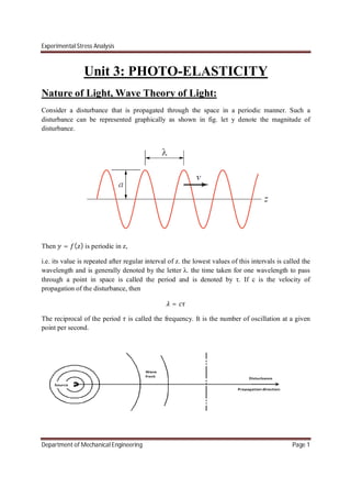
  • 1. Experimental Stress Analysis Department of Mechanical Engineering Page 1 Unit 3: PHOTO-ELASTICITY Nature of Light, Wave Theory of Light: Consider a disturbance that is propagated through the space in a periodic manner. Such a disturbance can be represented graphically as shown in fig. let y denote the magnitude of disturbance. Then = ( ) is periodic in z, i.e. its value is repeated after regular interval of z. the lowest values of this intervals is called the wavelength and is generally denoted by the letter λ. the time taken for one wavelength to pass through a point in space is called the period and is denoted by τ. If c is the velocity of propagation of the disturbance, then = The reciprocal of the period is called the frequency. It is the number of oscillation at a given point per second.
  • 2. Experimental Stress Analysis Department of Mechanical Engineering Page 2 Let disturbance originate from the point source. The disturbance travel outwards in all directions and if the medium is isotropic, the speed of propagation of these disturbances will be the same in all directions. Consequently, the disturbance travels in the form of diverging spherical waves. The locus of points having the same magnitude of disturbance is known as a wave-front, and in this particular case, the wave fronts are surface of concentric spheres with the source as centre. As this spherical wave s expands outwards, the radius becomes larger and any finite portion of the wave-front tends to become a plane. The direction of propagation of the disturbance would be perpendicular to the plane and is called the wave normal (transverse disturbance). The disturbance itself could be either perpendicular to the wave normal or in the direction of the wave normal (longitudinal disturbance). Consider a plane wave propagating in the z direction with velocity c. the wave front is parallel to the xy-plane. At time t=0, let the disturbance y be given by the equation = ( )……………….(2) After a time t, the disturbance will have travelled a distance ct and the graph shown in fig 1 will have shifted parallel to itself by a distance ct. Hence, the disturbance at a point z=z’+ct at time t is the same as the disturbance at z=z’ at time t=0. In other words, from eq 2, the disturbance at point z at time t is the same as the disturbance that existed at z-ct at time t=0, i.e. ( − ). Hence, the disturbance at z at time t can be written as = ( − ) … … … …… … … … . . (3) This is the fundamental equation of a plane wave travelling forward in the z-direction. Similarly, for a plane wave travelling backward, the fundamental equation is = ( + ) … … … …… … … … . . (4) If the disturbance is periodic, then the function ( ) is periodic in z. Eq 3 and 4 represents the plane waves can easily be seen since z= constant represents a plane parallel to the xy-plane and on this plane the disturbance y has a uniform magnitude. Similarly, the fundamental equation of a plane wave propagating in a direction with direction cosines (l,m,n) is = ( + + − )… … … … … … … … . . (5) Because, the equation + + = represents a plane whose normal has direction cosines (l,m,n) and on this plane the disturbance g has a uniform magnitude at a given time. A function ( ) which is periodic in z, the period being , can be expanded in a Fourier series as
  • 3. Experimental Stress Analysis Department of Mechanical Engineering Page 3 ( ) = + cos 2 ( +∈ )… … … … … … …… . . (6) For a periodic wave travelling forward with a velocity c, the Fourier expansion will be ( − ) = + cos 2 ( − +∈ )… … … … … … … … . . (7) The first vibratory component of the series, i.e. cos ( − +∈ ) is termed the fundamental simple form of a plane harmonic wave. In subsequent discussions, the typical fundamental light- wave propagating in the z-direction will be taken in the form = cos 2 ( − +∈)… … … … … … … … . . (8) The constant A is called the amplitude and the quantity ( − +∈) is called the phase. Light-waves belong to the class of transverse wave and the disturbance can be represented by means of a vector called the light vector. This light vector is perpendicular to the direction of propagation. Light is known to be an electromagnetic disturbance propagated through space and two vectors, namely the electric force vector H are associated with it. These two vectors are mutually perpendicular and either of these can be taken as the fundamental light vector. According to eq 8, the fundamental eq for light-wave (plane wave) travelling in the z-direction is = cos 2 ( − +∈) For a given value of z, the above eq can be written as
  • 4. Experimental Stress Analysis Department of Mechanical Engineering Page 4 = cos +∈ ……………………… (a) Where ∈ is some constant. From eq 1 1 = = Where is the frequency. This can be stated as the number of wavelengths travelled per second. 2 expresses the quantity in radians per second and is called the circular frequency. Denoting the circular frequency by , eq A becomes = cos( +∈ )…………….(b) Instead of cosine function sin function can also be used to represent a plane harmonic wave, i.e = sin( +∈ )………………(c) The frequency of a light wave determines that quality which the eye recognizes as color. The lowest frequency which the human eye can recognize as light is about 390*1012 and this corresponds to deep red color. The highest frequency is about 770*1012 corresponding to deep violet. Between these two frequencies, one finds the colors arranged as violet, indigo, blue, green, yellow, orange, and red. The gradation from one color to next is smooth and not abrupt. When these colors are spread out to form a continues band, it is called a spectrum. Light corresponding to one particular frequency and one color is said to be homogeneous or monochromatic. It was stated that light-wave belongs to the class of transverse waves and the disturbance can be represented by means of a vector called the light vector. In ordinary light, the tip of the light- vector describes a random vibratory motion in a plane transverse to the direction of propagation. If the tip of the light-vector is forced to follow a definite law, the light is said to be polarized. For example, if the tip is constrained to lie on the circumference of a circle, it is said to be circularly polarized. If the tip describes an ellipse, it is elliptically polarized. If the light vector is parallel to a given direction in the wave-front, it is said to be linearly or plane polarized. These are shown in fig. if the tip of the light-vector in fig (a) describes the circle in a counter-clockwise direction as shown, then it is said to be right handedly circularly polarized. On the other hand, if the path is transverse in a clockwise direction, then it is left-handedly circularly polarized. This notation is adopted so as to be consistent with the right-handed coordinate system. The positive z-axis is away from the source and the vibrations are in planes parallel to the xy-plane.
  • 5. Experimental Stress Analysis Department of Mechanical Engineering Page 5 Similarly, one can speak of right-handedly or left-handedly elliptically polarized light. It is easily observed that an elliptically polarized light is the most general form of polarized light since a circle can be considered as an ellipse with the major and minor axes being equal. Similarly, a straight line is a degenerated form of an ellipse with the minor axis being equal to zero. Optically isotropic: Refractive index is same for all direction in the material. Therefore light propagate with the same velocity in all direction. Optically Anisotropic: the ability to resolve the light vector into two orthogonal components and transmit the components with different velocity in different direction. Such material is known as double refracting or bifringement material. This type of properties is known as optically anisotropic property. Double Refraction: when a beam of un-polarized light is incident on the crystalline material , the beam upon entering the material get split into two component of plane polarized light. This
  • 6. Experimental Stress Analysis Department of Mechanical Engineering Page 6 phenomenon is known as double refraction and the material exhibiting this behavior is known as double refractive material. Wave plate: certain crystalline materials have the ability to resolve the light vectors into two orthogonal components and transmit each one of them in different speed and phase. This phase difference is proportional to the thickness of the plate. A typical wave plate is as shown in fig. The wave plates are of two types quarter wave plate(Q.W.P) and half wave plate(H.W.P), depending on the path difference(andrespectively produce between the two orthogonal components. Photo-elasticity: photo-elasticity is a stress analysis technique using the relative retardation b/w two components of light vector along the directions of two principle stresses at a point on a photo-elastic model. Photo-elastic model: A photo-elastic model is a transparent material possessing the property of temporary double refraction. Without external load, the model is isotropic and when it is loaded, refractive index changes along the directions of principle stresses in the model.
  • 7. Experimental Stress Analysis Department of Mechanical Engineering Page 7 There are many transparent, non-crystalline materials which are optically isotropic when free of stress but become optically anisotropic after the application of stress. This behavior is known as double refraction and the materials exhibits this behavior are known as photo-elastic materials. As long as the loads are maintained on the photo-elastic materials, it exhibits the behavior of temporary double refraction and the material becomes again isotropic after the removal of loads. Stress optic law: fig 1 shows a unstressed thin disc of a photo-elastic model. The refractive index of this material in any direction is n0. This thin disc is subjected to loads such that the principal stresses developed at a point o are and as shown in fig 2. The refractive index of material changes in the direction of to the value n1 and n2 in the direction . These changes in refractive idiocies are linearly proportional to the stresses. − = + …….(1) − = + …….(2) Where and are the principal stresses at a point in a material under plane stress condition. is refractive index of unstressed model. are the refractive index of stressed model associated with the directions of principal stress and . , are stress optic co-efficient. These changes is refractive index can be used as the basis for a stress measurement technique I,e photo-elasticity. eq(2)-eq(1) − = ( − )( − ) − = ( − )…….(3)
  • 8. Experimental Stress Analysis Department of Mechanical Engineering Page 8 Where, − = c If > and velocity of propagation of light wave associated with principle stress is greater than the velocity of propagation of light wave associated with principal stress is known as positive bifringence. A photo-elastic model behaves like a wave plate and it can be used to relate the relative retardation Δ to changes in the refractive index in the material due to stress. If a beam of plane polarized light is passed through the thin sheet of photo-elastic material at normal incidence as shown, then relative retardation Δ between the two components of light vector along each of principal stress directions can be obtained by ∆= ( − )…………..(4) h= thickness of model =magnitude of relative retardation b/w two components of light beam propagating in directions perpendicular to and . Eq 4 shows that relative retardation is linearly proportional to ( − ), h and inversely proportional to wavelength of light being used. The relative stress optic co-efficient c is assumed as a material constant ( − ) = ∆ ∗ ∗ …………(5) ∆ = , , = = ( − ) = ℎ
  • 9. Experimental Stress Analysis Department of Mechanical Engineering Page 9 stress fringe value is a property of the model material and it is determined by calibration. If photo-elastic model material exhibits a perfectly linear elastic behavior, the difference in principal strain ∈ −∈ can also be measured by establishing the value N, relative retardation ∈ = 1 ( − ) ∈ = 1 ( − ) ∈ −∈ = 1 (1 + )( − ) ∈ −∈ = 1 (1 + ) ℎ ∈ −∈ = ∈ ℎ ∈ = (1 + ) ∈ = Types of polariscopes: We have two types of polariscopes 1) Plane polariscopes, 2) Circular polariscopes 1) Plane polariscope: It is the simplest model or optical system used in photo-elasticity. It consists of two linear polarizer’s and a light source as shown in the figure. The linear polarizer nearest to the light source is called polarizer. While the second linear polarizer is away from the light source called analyzer. Here the two axes of the polarizer’s always cross. Hence no light is transmitted through the analyzer and produce dark field. The model is inserted and viewed through analyzer. The polarizer is kept perpendicular to the axes of light propagation it transmits the light wave comes only in there axes. The analyzer is kept 90 deg to the polarizer and it transmit the light waves in there axes.
  • 10. Experimental Stress Analysis Department of Mechanical Engineering Page 10 2) Circular polariscopes It employs circularly polarized light. The first element following light source is called polarizer. It converts ordinary light into plane polarized light. The second wave plate is quarter wave plate with an angle π/4 to the plane of polarization. This quarter wave plate’s convert’s plane polarized light into circularly polarized light. The second quarter wave plate is kept between the analyzer and model. The second quarter wave plate converts circularly polarized light into plane polarized light. The last element is analyzer which extinguishes the light.
  • 11. Experimental Stress Analysis Department of Mechanical Engineering Page 11 Isoclinic and Isochromatics: Consider the arrangement shown in fig. i.e., monochromatic light source, polarizer, model is in plane state of stress, and analyzer, is a second polarizing element kept 90 deg to polarizer axes. We should assume that through a suitable optical arrangement, the image of the model is projected on the screen. The polarizer and analyzer are always kept crossed, but their combined orientation can be arbitrary. When a model is stressed, it behaves as a crystal and at the point where the ray passes, the polarizing axis coincide with the principal stress axes , at that point. In general, the polarizer makes an angle with axes. If the polarizer coincides with either then the plane polarized light incident on the model at that point will emerge as a plane polarized light. Since the analyzer is kept crossed with respect to polarizer, the light coming out of the analyzer is zero. Consequently, at all those point of model, where the directions of the principal stress happen to coincide with the particular orientation of the polarizer analyzer combination , the light coming out of the analyzer will be zero. If the polarizer analyzer combination happens to coincide with the directions of , stresses at one point of the model, then in general, there will be a locus of points in the model along which this condition is satisfied. This is so because, in general, the stresses are distributed in a continuous manner in the model. The locus of points where the directions of the principal stresses coincide with a particular orientation of the polarizer-analyzer combination is known as Isoclinic’s. Suppose at a particular point of the model, the values of , are such as to cause a relative phase difference of 2mπ where m is an integer. The relative phase difference is related to
  • 12. Experimental Stress Analysis Department of Mechanical Engineering Page 12 − . When the relative phase difference is 2mπ, the model behaves as a full wave plate at that particular point. The discussion on crystal optics shown that an incident linearly polarized light on a full-wave plate emerges as a linearly polarized light and is cut off by the analyzer, because of its crossed position. Therefore, at all those points of the model where the values of − are such as to cause a relative phase difference of 2mπ, the intensity of light on the screen will be zero. On the screen, a series of dark bands corresponding to the loci of these points are observed. These dark bands or fringes are known as Isochromatics. An Isochromatics is a locus of points where the values of − are such as to cause a relative phase difference of 2mπ, when background is dark. Effect of Stressed Model in Plane Polariscopes (Dark Field Set up) It consists of two linear polarizer’s and a light source as shown in the figure. The linear polarizer nearest to the light source is called polarizer. It transmits the plane polarized light in there axis. While the second linear polarizer is away from the light source called analyzer. Here the two axes of the polarizer’s always cross. Hence no light is transmitted through the analyzer and produce dark field. The model is inserted and viewed through analyzer. The polarizer is kept perpendicular to the axes of light propagation it transmits the light wave comes only in there axes. The analyzer is kept 90 deg to the polarizer and it transmit the light waves in there axes. The component of light vector transmitted by the polarizer is = cos The light vector when incident on the model is resolved into two components along principle stress direction. = cos cos = cos sin and are incident on one side of photo-elastic model. These two components of the light vector propagate through the stressed model at different velocities. As a result, when these two components emerge from the model, these are out of phase. Upon leavening the model, the two vibrating components acquire a relative phase difference of Δ. We shall assume that leads . Hence, upon leavening the model, the vibrating components are = cos( + Δ) cos = cos sin
  • 13. Experimental Stress Analysis Department of Mechanical Engineering Page 13
  • 14. Experimental Stress Analysis Department of Mechanical Engineering Page 14 On entering analyzer, only the components along are allowed to emerge = sin − cos = cos( + Δ) cos sin − cos sin cos = cos sin [cos( + Δ) − cos ] = 2 sin 2 [cos cos∆ − sin sin ∆ − cos ] = 2 sin 2 [cos (cos ∆ − 1) − sin sin ∆] = 2 sin 2 −2cos ∆ 2 − 2sin sin ∆ 2 ∆ 2 = − sin 2 ∆ 2 cos ∆ 2 + sin ∆ 2 = − sin2 ∆ 2 sin + ∆ 2 = − sin + ∆ 2 = sin2 ∆ is the amplitude of emerging light vector. A measure of intensity of light is given by the square of amplitude. In our case, the intensity is = = sin 2 ∆ 2 Intensity of light coming out of analyzer is zero under two conditions (1) When = 90 (2) When ∆= 2 ( = 0,1,2,3 … . ) First condition tells that light extinction occur at a point when direction of principal stresses coincide with the direction of polarizer and analyzer. The locus of point when this happens is called the Isoclinic’s. Second condition tells that light extinction occur at a point when the relative phase difference is equal to2 . The locus of point where this occurs is called Isochromatics.
  • 15. Experimental Stress Analysis Department of Mechanical Engineering Page 15 Effect of Stressed Model in Circular Polariscopes under Dark Field Arrangement: It employs circularly polarized light. The first element following light source is called polarizer. It converts ordinary light into plane polarized light. The second wave plate is quarter wave plate with an angle π/4 to the plane of polarization. This quarter wave plate’s convert’s plane polarized light into circularly polarized light. The second quarter wave plate is kept between the analyzer and model. The second quarter wave plate converts circularly polarized light into plane polarized light. The last element is analyzer which extinguishes the light. The light vector emerging out of polarizer = cos Light vector entering first Q.W.P = cos45 = cos45 = cos 1 √2 = cos 1 √2
  • 16. Experimental Stress Analysis Department of Mechanical Engineering Page 16 The two vectors travels with a different velocity along the Q.W.P so they will have an angular phase shift of /2. The light vector leavening first Q.W.P = cos( + /2) √2 = −sin( ) √2 = cos( ) √2 Here Ist light vector gains the phase shift of /2 because it travels faster than the second light vector. The light vector entering the model = cos − sin = −sin( ) ∗ √2 ∗ cos − cos( ) ∗ √2 ∗ sin = − √2 {sin( )cos + cos( )sin } = − √2 {sin( + )} = sin + cos = sin( ) ∗ √2 ∗ sin − cos( ) ∗ √2 ∗ cos = √2 {sin( ) sin −cos( )cos }
  • 17. Experimental Stress Analysis Department of Mechanical Engineering Page 17 = √2 {cos( + )} The light vector leavening the model will have an angular phase shift = − √2 {sin( + + ∆)} = + √2 {cos( + )} The light vector entering second Q.W.P = cos + sin = − √2 {sin( + + ∆)}cos + √2 {cos( + )} sin = cos − sin = √2 {cos( + )}cos + √2 {sin( + + ∆)} sin The light vector leaves the second Q.W.P with a phase difference of  = − √2 {sin( + + ∆)}cos + √2 {cos( + )} sin 
  • 18. Experimental Stress Analysis Department of Mechanical Engineering Page 18 = √2 {cos( + + /2)}cos + √2 {sin( + + ∆ + /2)} sin = − √2 {sin( + )} cos + √2 {cos( + + ∆)} sin The light vector entering the analyzer  = cos45 − cos45 = 1 √2 − √2 {sin( + + ∆)} cos + √2 {cos( + )}sin + √2 {sin( + )}cos − √2 {cos( + + ∆)}sin = 2 [{cos( + )}sin + {sin( + )}cos − {cos( + + ∆)}sin + {sin( + + ∆)}cos ] = 2 [{sin( + 2 )} − {sin( + 2 + ∆)}] = cos + 2 + ∆ 2 sin ∆ 2 = cos + 2 + ∆ 2 = = sin ∆ 2
  • 19. Experimental Stress Analysis Department of Mechanical Engineering Page 19 Since the intensity of light is square of amplitude the frequency is very high any extinction produced by this cannot be detected by photographic equipment hence isoclinic are eliminated from the fringe pattern, observed with circular polarizer. The fringe pattern associated with the pattern is Isochromatics fringe pattern. Thus circular polariscopes eliminates isoclinic fringe pattern. Thus circular polariscopes eliminates isoclinic’s fringe pattern and returns only Isochromatics fringe pattern. Effect of Stressed Model in Circular Polariscope under Dark Field Arrangement: Consider axes of polarizer and analyzers are parallel. Thus = cos45 + cos45 = 1 √2 − √2 {sin( + + ∆)} cos + √2 {cos( + )}sin − √2 {sin( + )}cos + √2 {cos( + + ∆)}sin = 2 [{cos( + )}sin − {sin( + )}cos + {cos( + + ∆)}sin − {sin( + + ∆)}cos ] = 2 [−{sin( )} − {sin( + ∆)}] = − 2 ∗ 2 ∗ sin + ∆ 2 ∗ cos ∆ 2
  • 20. Experimental Stress Analysis Department of Mechanical Engineering Page 20 = − sin + ∆ 2 ∗ cos ∆ 2 = − sin + ∆ 2 = cos ∆ 2 = = cos ∆ 2 For extinction to occur ∆ 2 = (2 + 1) 2 = 0,1,2, …. = ∆ 2 = + 1 2 Hence the order of first fringe observed in a light field polariscopes is ½ which corresponds to n=0. The higher order fringe will be 3/2, 5/2, 7/2,….etc. therefore by using dark and bright field setup of the circular polariscopes, it is possible to obtain the fringe order to the nearest ½ order. Method of compensation Consider any one point in the model, the relative retardation is between 3 to 3.5as observed by the bright and dark field setups. Let us assume that the value is 3.36this is equal to 3.36 fringe order. The decimal part i.e., 0.36 of this value is called the fractional fringe order at that point. The compensation means raising the existing value 3.36 to 4 or reducing the value to 3.0. (1) Babinet-Soleil compensator
  • 21. Experimental Stress Analysis Department of Mechanical Engineering Page 21 It consists of two quartz wedges cut similarly with respect to their optical axes. A and B are the two wedges with their fast axes similarly oriented, so that the two wedges together form one rectangular piece of uniform thickness. By moving one wedge with respect to the other, the thickness of the combination over this portion can be varied. Next to the wedge combination is a quartz plate C of uniform thickness. The fast axes of this are right angle to the fast axes of wedge combination. The retardation given by the plate c can be cancelled partially or fully by varying the thickness of the wedge combination. Hence by adjusting the overall thickness of the wedge combination the compensator can add or subtracts the relative retardation within a given range. The micrometer screw is calibrated in number of wavelengths of retardation added or subtracted along marked axes of compensator. The compensator is kept before or after the model and is oriented along the principal stress axis at the point of interest in the model. When t1=t2 no relative retardation take place, however for t2>t1 positive and t1>t2, negative retardation can be produced over the whole area of the compensator plate. (2) The Tardy Method of Compensation The Tardy method of compensator is generally preferred over the Babinet-Soleil method since no auxiliary equipment is required and analyzer of polariscopes is aligned with the direction of the principal stresses at that point of interest and all other elements of polariscopes are rotated relative to polarizer so that standard dark field polariscopes exist. Then the analyzer alone is rotated to obtain extinction. The rotation of analyzer gives fractional fringe order.
  • 22. Experimental Stress Analysis Department of Mechanical Engineering Page 22  The light vector emerging out from the second Q.W.P is = − √2 sin − 4 + ∆ cos − 4 + √2 cos − 4 sin − 4  = − 2 sin − 4 + ∆ − 2 cos − 4  = − √2 sin − 4 cos − 4 + √2 cos − 4 + ∆ sin − 4 = − 2 sin − 4 − 2 cos − 4 + ∆ Let be the angle through which analyzer should be rotated to obtain extinction i.e., = 0 then, = cos 4 + − cos 4 − = − 2 sin − 4 + ∆ − 2 cos − 4 cos 4 + − − 2 sin − 4 − 2 cos − 4 + ∆ cos 4 − = − 2 sin − 4 + ∆ cos 4 + + cos − 4 cos 4 + − cos 4 − sin − 4 + cos 4 − cos − 4 + ∆ After simplification we will have
  • 23. Experimental Stress Analysis Department of Mechanical Engineering Page 23 = sin + ∆ 2 sin ∆ 2 − If intensity is zero sin ∆ 2 − = 0 ∆ 2 − = ∆ 2 = + Where m = 0 1, 2, 3…. N = ∆ 2 = + If the analyzer is rotated in the opposite direction then N = ∆ 2 = ( + 1) − A plane polariscopes arrangement is first employed so that are isoclinic fringe will pass through the point of interest. Now a plane polariscopes is converted to circular polariscopes dark field arrangement. Then analyzer rotated until extinction occurs at a point of interest. Eg: if analyzer rotated through an angle, such that second order i.e, m=2 fringe passes through the point of interest then directly fringe order is given by N = ∆ 2 = + = 2 + If analyzer rotate in opposite direction N = ∆ 2 = ( + 1) − = 3 − (3) Friedel’s Method
  • 24. Experimental Stress Analysis Department of Mechanical Engineering Page 24 Steps followed for doing Friedel’s method 1. Remove first Q.W.P 2. Rotate polarizer and analyzer so that their axes makes an angle of 45 deg with principle direction in the model at that point of interest. 3. Rotate second Q.W.P until one axes is parallel to axes of polarizer. 4. Rotate the analyzer until extinction is obtained at the point. The light vector emerging out of polarizer = cos Since polarizer is set 45 deg to axes of principle direction in model hence on entering the model the light vector is resolved into two components given by = cos45 = cos 1 √2 = cos45 = cos 1 √2 The model introduces a phase difference of therefore on leaving the model, the components of light vector becomes, = cos( + ∆) √2  = cos √2
  • 25. Experimental Stress Analysis Department of Mechanical Engineering Page 25 the fast axes of Q.W.P is set 90 deg to polarizer axes. Hence on entering the Q.W.P the light components become, = cos45 − cos45 = 2 {cos( + ∆) − cos } = cos45 + cos45 = 2 {cos( + ∆) + cos } On leaving the Q.W.P the Q.W.P introduce phase difference of hence on leaving the Q.W.P. the light vector becomes = 2 cos + ∆ + 2 − cos + 2 = 2 {− sin( + ∆) + sin } = 2 {cos( + ∆) + cos } The analyzer is rotated through an angle of to obtain extinction at the point of interest. Light transmitted through analyzer is = cos − sin = − 2 [sin( + ∆) − sin ] cos − 2 [cos( + ∆) + cos ]sin = − 2 2cos + ∆ 2 sin ∆ 2 cos + 2 cos + ∆ 2 cos ∆ 2 sin When intensity of light is zero = sin ∆ 2 cos + cos ∆ 2 sin = 0 sin ∆ 2 cos + cos ∆ 2 sin = 0 sin ∆ 2 + = 0 ∆ 2 + = = 0,1,2,…
  • 26. Experimental Stress Analysis Department of Mechanical Engineering Page 26 = ∆ 2 = − Fringe Sharpening by Partial Mirror To decrease the band width of Isochromatics fringes ordinary circular polariscopes is modified by inserting partial mirrors on both side of the model and both are parallel to the model. We know that intensity of light = sin ∆ 2 = sin ∆ 2 The intensity of light is modified by the transmittance (T) and refractance (R) For ray 1, the intensity of light is lost by reflection from the partial mirror and resultant I will become = R sin ∆ 2 = sin ∆ 2 Similarly Ray 3 passes through the model 3 times and combined to yield intensity = R sin 3∆ 2 For mth ray = R( ) sin ∆ 2 The intensities , , add arithmetically the intensity of sharpened Isochromatics fringe is given by
  • 27. Experimental Stress Analysis Department of Mechanical Engineering Page 27 = R( ) sin ∆ 2 The loss of intensity can be minimized by selecting mirror co-efficient R and T. Assuming mirrors are perfect T+R=1 T=1-R R( ) ≤ 1 Intensity of sharpened fringe pattern is decrease by R( ) compare to ordinary fringe pattern. In actual practice rays are not inclined as shown: these rays propagate back and forth through the model at the same point of the model number of times and intensity of ray progressively diminishes. Fringe Multiplication by Partial Mirror Fringe multiplication is concerned important since standard method of compensation used to evaluate the fraction fringe order are time consuming and in some case also inaccurate. Fringe multiplication is a compensation technique where the fractional orders of the fringe can be determined simultaneously at all points on the model. Partial mirror can be used to multiply the number of Isochromatics fringes if one partial mirror is placed parallel to the photo elastic model and the other partial mirror is placed slightly inclined
  • 28. Experimental Stress Analysis Department of Mechanical Engineering Page 28 with the plane of photo elastic model as shown in fig. partial mirror PM I is parallel to model M but partial mirror PM II is slightly inclined with the model at an angle Ray 1 emerges from partial mirror II, traversing two times the partial mirrors and one time through the model, intensity of light for ray 1 is = sin ∆ 2 = R sin 3∆ 2 = R sin 5∆ 2 = R sin ∆ 2 Different rays are inclined with the axis of polariscopes, at angle 0, 246as shown, each ray gets isolated and passes out from different points of the model. Any of these rays can be observed at the proper image point of focal field lens. As is obvious from the intensity equations above, Isochromatics fringe patterns can be multiplied by 1, 3, 5, 7 and so on. Fringes are not only multiplied but they are sharpened at the same time. Fringe order recorded with ray 1 are 0, 0.5, 1, 1.5, 2, 2.5….. Fringe order recorded with ray 3 is 0, 1/6, 1/3, ½, 2/3, 5/6, 1… Similarly fringe orders recorded with ray 5 are 0.1, 0.2, and 0 .3, 0.4… As tilting angle increases fringes also increases thus fringe multiplication by this method is accomplished by considerable loss in the light intensity I of the multiplied fringe pattern as compared with the ordinary fringe pattern. Calibration Techniques The photo elastic material has to be calibrated to determine the material fringe value so as to convert the fringe orders into stresses. The following methods may be used to calibrate a photo elastic model. 1. Simple tensile specimen:
  • 29. Experimental Stress Analysis Department of Mechanical Engineering Page 29 If we prepare a simple tensile specimen as shown in fig(a), whose width is w and thickness h, then under load P, the uniform stress in the test specimen is − = ℎ⁄ Then = 0 Applying stress optic law, we get − = ℎ ℎ = ℎ Hence, = In the tensile specimen, we get escaping type of fringes, i.e. as the load is increased from zero, successive fringe appear in the field of view and disappear as the load is increased. Generally a graph is plotted between the load applied P and fringe order N as shown in fig (b) and its slope is determined, which is substituted in above eq to determine . In this method load P has to be adjusted to have a full fringe order in the field of view. In another technique, the Tardy’s method of compensation is used, where for a particular load P the extinction angle are plotted against the applied stress . Then by knowing the slope of the curve, we have = . ℎ. 180
  • 30. Experimental Stress Analysis Department of Mechanical Engineering Page 30 In a similar way a compensation test piece may also be used. 2. Beam under pure bending: A rectangular beam of thickness h and depth w as shown in fig (a) may be used and subjected to pure bending to determine . Pure bending in the beam may be produced by applying equal load P at a distance a from the ends of a beam of length l as shown. The uniform bending moment M in the middle portion of the beam is = The stress in the beam are = . = ℎ 12 2 = ℎ 6 , = 0 Hence, = = 6 A graph is plotted between P and N and the slope of the curve is substituted in above eq to determine . Here we get non-escaping type of fringes. The fringe pattern in the pure bending calibration specimen are shown in fig below
  • 31. Experimental Stress Analysis Department of Mechanical Engineering Page 31 3. Circular disc under diametral compression: For a circular disc of diameter D and thickness h as shown in fig (a), when subjected to a diametral compressive load P, the stresses along the horizontal diameter are given by = = 2 ℎ − 4 + 4 = = − 2 ℎ 4 [ + 4 ] − 1 = 0 − = 8 ℎ [1 − 4( ⁄ ) ] [1 + 4( ⁄ ) ]
  • 32. Experimental Stress Analysis Department of Mechanical Engineering Page 32 At the center, i.e. = 0, = 2 ℎ = − 6 ℎ Hence − = = = 8 By knowing the value of P for a particular fringe order N at the center of disc, a graph can be plotted, whose slope is substituted in above eq to determine the value of . The fringe pattern in the circular disc is shown in fig below