The Stellar Magnitude System

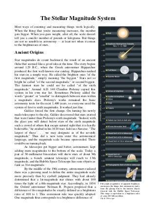
1. The Stellar Magnitude System
Most ways of counting and measuring things work logically.
When the thing that you're measuring increases, the number
gets bigger. When you gain weight, after all, the scale doesn't
tell you a smaller number of pounds or kilograms. But things
are not so sensible in astronomy — at least not when it comes
to the brightnesses of stars.
Ancient Origins
Star magnitudes do count backward, the result of an ancient
fluke that seemed like a good idea at the time. The story begins
around 129 B.C., when the Greek astronomer Hipparchus
produced the first well-known star catalog. Hipparchus ranked
his stars in a simple way. He called the brightest ones "of the
first magnitude," simply meaning "the biggest." Stars not so
bright he called "of the second magnitude," or second biggest.
The faintest stars he could see he called "of the sixth
magnitude." Around A.D. 140 Claudius Ptolemy copied this
system in his own star list. Sometimes Ptolemy added the
words "greater" or "smaller" to distinguish between stars within
a magnitude class. Ptolemy's works remained the basic
astronomy texts for the next 1,400 years, so everyone used the
system of first to sixth magnitudes. It worked just fine.
Galileo forced the first change. On turning his newly
made telescopes to the sky, Galileo discovered that stars existed
that were fainter than Ptolemy's sixth magnitude. "Indeed, with
the glass you will detect below stars of the sixth magnitude
such a crowd of others that escape natural sight that it is hardly
believable," he exulted in his 1610 tract Sidereus Nuncius. "The
largest of these . . . we may designate as of the seventh
magnitude." Thus did a new term enter the astronomical
language, and the magnitude scale became open-ended. There
could be no turning back.
As telescopes got bigger and better, astronomers kept
adding more magnitudes to the bottom of the scale. Today a
pair of 50-millimeter binoculars will show stars of about 9th
magnitude, a 6-inch amateur telescope will reach to 13th
magnitude, and the Hubble Space Telescope has seen objects as
faint as 31st magnitude.
By the middle of the 19th century, astronomers realized
there was a pressing need to define the entire magnitude scale
more precisely than by eyeball judgment. They had already
determined that a 1st-magnitude star shines with about 100
times the light of a 6th-magnitude star. Accordingly, in 1856
the Oxford astronomer Norman R. Pogson proposed that a
difference of five magnitudes be exactly defined as a brightness
ratio of 100 to 1. This convenient rule was quickly adopted.
One magnitude thus corresponds to a brightness difference of
Fifty-eight magnitudes of apparent brightness
encompass the things that astronomers study,
from the glaring Sun to the faintest objects
detected with the Hubble Space Telescope.
This range is equivalent to a brightness ratio
of some 200 billion trillion.
Sky & Telescope

2. exactly the fifth root of 100, or very close to 2.512 — a value
known as the Pogson ratio.
The brightness we observe of a star (or flux) is the
amount of energy received per second per square meter and it
relates to the stars luminosity with the formula:
𝑙 =
𝐿
4𝜋𝑟2
where r is the distance from earth to the star. This can be used to
define the apparent magnitude of a star. For two stars of
apparent magnitudes m1 nad m2 and brightnesses l1 and l2
respectively, we have:
𝑙1
𝑙2
= √100
5 (𝑚2−𝑚1)
⇒ 𝑙𝑜𝑔 (
𝑙1
𝑙2
) = 𝑙𝑜𝑔 (√100
5 (𝑚2−𝑚1)
) ⇒
𝑙𝑜𝑔 (
𝑙1
𝑙2
) =
𝑚2 − 𝑚1
5
𝑙𝑜𝑔100 ⇒
The resulting magnitude scale is logarithmic, in neat
agreement with the 1850s belief that all human senses are
logarithmic in their response to stimuli. The decibel scale for
rating loudness was likewise made logarithmic.
Alas, it's not quite so, not for brightness, sound, or
anything else. Our perceptions of the world follow power-law
curves, not logarithmic ones. Thus a star of magnitude 3.0 does
not in fact look exactly halfway in brightness between 2.0 and
4.0. It looks a little fainter than that. The star that looks halfway
between 2.0 and 4.0 will be about magnitude 2.8. The wider the
magnitude gap, the greater this discrepancy. Accordingly, Sky &
Telescope's computer-drawn sky maps use star dots that are
sized according to a power-law relation.
Now that star magnitudes were ranked on a precise
mathematical scale, however ill-fitting, another problem became
unavoidable. Some "1st-magnitude" stars were a whole lot
brighter than others. Astronomers had no choice but to extend the scale out to brighter values as
well as faint ones. Thus Rigel, Capella, Arcturus, and Vega are magnitude 0 (by definition), an
awkward statement that sounds like they have no brightness at all! But it was too late to start over.
The magnitude scale extends farther into negative numbers: Sirius shines at magnitude –1.5, Venus
reaches –4.4, the full Moon is about –12.5, and the Sun blazes at magnitude –26.7.
Other Colors, Other Magnitudes
By the late 19th century astronomers were using photography to record the sky and measure star
brightnesses, and a new problem cropped up. Some stars showing the same brightness to the eye
showed different brightnesses on film, and vice versa. Compared to the eye, photographic
emulsions were more sensitive to blue light and less so to red light. Accordingly, two separate
scales were devised. Visual magnitude, or mvis, described how a star looked to the eye.
Photographic magnitude, or mpg, referred to star images on blue-sensitive black-and-white film.
These are now abbreviated mv and mp, respectively.
The Meaning of Magnitudes
This difference
in magnitude...
...means this ratio
in brightness
0 1 to 1
0.1 1.1 to 1
0.2 1.2 to 1
0.3 1.3 to 1
0.4 1.4 to 1
0.5 1.6 to 1
1.0 2.5 to 1
2 6.3 to 1
3 16 to 1
4 40 to 1
5 100 to 1
10 10,000 to 1
20 100,000,000 to 1
𝑚1 − 𝑚2 = −2,5𝑙𝑜𝑔 (
𝑙1
𝑙2
) (1)

3. This complication turned out to be a blessing in
disguise. The difference between a star's photographic
and visual magnitude was a convenient measure of the
star's color. The difference between the two kinds of
magnitude was named the "color index." Its value is
increasingly positive for yellow, orange, and red stars,
and negative for blue ones.
But different photographic emulsions have
different spectral responses! And people's eyes differ
too. For one thing, your eye lenses turn yellow with
age; old people see the world through yellow filters.
Magnitude systems designed for different wavelength
ranges had to be more clearly defined than this.
Today, precise magnitudes are specified by what
a standard photoelectric photometer sees through standard color filters. Several photometric systems
have been devised; the most familiar is called UBV after the three filters most commonly used. U
encompasses the near-ultraviolet, B is blue, and V corresponds fairly closely to the old visual
magnitude; its wide peak is in the yellow-green band, where the eye is most sensitive.
Color index is now defined as the B magnitude minus the V magnitude. A pure white star
has a B-V of about 0.2, our yellow Sun is 0.63, orange-red Betelgeuse is 1.85, and the bluest star
believed possible is –0.4, pale blue-white.
So successful was the
UBV system that it was extended
redward with R and I filters to
define standard red and near-
infrared magnitudes. Hence it is
sometimes called UBVRI.
Infrared astronomers have carried
it to still longer wavelengths,
picking up alphabetically after I to
define the J, K, L, M, N, and Q
bands. These were chosen to
match the wavelengths of infrared
"windows" in the Earth's
atmosphere — wavelengths at
which water vapor does not
entirely absorb starlight.
In all wavebands, the bright star
Vega has been chosen (arbitrarily)
to define magnitude 0.0. Since
Vega is dimmer at infrared
wavelengths than in visible light,
infrared magnitudes are, by
definition and quite artificially,
"brighter" than their visual
counterparts.
Appearance and Reality
What, then, is an object's real brightness? How much total energy is it sending to us at all
wavelengths combined, visible and invisible? The answer is called the bolometric magnitude, mbol,
The bandpasses of the standard UBVRI color filters,
along with the spectrum of a typical blue-white star.
Sky & Telescope
The color index (CI) is usually
CI = mB - mV
where mB is the blue color magnitude of the star and mV the
visible color magnitude. As the magnitude increases with
decreasing brightness a star with a smaller index will be
more blue and a star with a larger index more red. The
following table should help you do the translation:
Color Index Spectral Class Color
-0.33 O5 Blue
-0.17 B5 Blue-white
0.15 A5 White with bluish tinge
0.44 F5 Yellow-White
0.68 G5 Yellow
1.15 K5 Orange
1.64 M5 Red
This table is only valid for the B-V (or Blue minus Visible)
color index. Often astronomers use other color indexes such
as U-B (Ultraviolet minus Blue) or H-K (H-band minus K-
band) indexes.

4. because total radiation was once measured with a device called a bolometer. The bolometric
magnitude has been called the God's-eye view of an object's true luster. Astrophysicists value it as
the true measure of an object's total energy emission as seen from Earth. The bolometric correction
tells how much brighter the bolometric magnitude is than the V magnitude. Its value is always
negative, because any star or object emits at least some radiation outside the visual portion of the
electromagnetic spectrum.
Up to now we've been dealing only with apparent magnitudes — how bright things look
from Earth. We don't know how intrinsically bright an object is until we also take its distance into
account. Thus astronomers created the absolute magnitude scale. An object's absolute magnitude
is simply how bright it would appear if placed at a standard distance of 10 parsecs (32.6 light-
years).
On the left-hand map of Canis Major, dot sizes indicate stars' apparent magnitudes; the dots
match the brightnesses of the stars as we see them. The right-hand version indicates the same stars'
absolute magnitudes — how bright they would appear if they were all placed at the same distance
(32.6 light-years) from Earth. Absolute magnitude is a measure of true stellar luminosity.
The absolute brightness of a star in relation with its apparent one would be:
𝑙 𝑎
𝑙 𝐴
=
𝐿
4𝜋𝑟2
𝐿
4𝜋𝑟𝐴
2
⇒
𝑙 𝑎
𝑙 𝐴
=
𝑟𝐴
2
𝑟2
⇒
𝑙 𝑎
𝑙 𝐴
=
100
𝑟2
, 𝑟 𝜎𝜀 𝑝𝑎𝑟𝑠𝑒𝑐𝑠
By inserting that to formula (1) we get:
𝑚 − 𝑀 = −2,5𝑙𝑜𝑔 (
𝑙 𝑎
𝑙 𝐴
) ⇒ 𝑚 − 𝑀 = −2,5𝑙𝑜𝑔 (
100
𝑟2
) ⇒ m − M = −2,5𝑙𝑜𝑔100 + 2,5𝑙𝑜𝑔(r2
) ⇒
Seen from this distance, the Sun would shine at an unimpressive visual magnitude 4.85.
Rigel would blaze at a dazzling –8, nearly as bright as the quarter Moon. The red dwarf Proxima
Centauri, the closest star to the solar system, would appear to be magnitude 15.6, the tiniest little
glimmer visible in a 16-inch telescope! Knowing absolute magnitudes makes plain how vastly
diverse are the objects that we casually lump together under the single word "star."
Absolute magnitudes are always written with a capital M, apparent magnitudes with a lower-
case m. Any type of apparent magnitude — photographic, bolometric, or whatever — can be
converted to an absolute magnitude.
(For comets and asteroids, a very different "absolute magnitude" is used. The standard here
is how bright the object would appear to an observer standing on the Sun if the object were one
astronomical unit away.)
So, is the magnitude system too complicated? Not at all. It has grown and evolved to fill
every brightness-measuring need exactly as required. Hipparcus would be thrilled.
𝑚 − 𝑀 = 5 log 𝑟 − 5

5. Black-body radiation (From Wikipedia, the free encyclopedia)
Black-body radiation is the type of electromagnetic radiation within or surrounding a body in
thermodynamic equilibrium with its environment, or emitted by a black body (an opaque and
non-reflective body) held at constant, uniform temperature. The radiation has a specific
spectrum and intensity that depends only on the temperature of the body.
A perfectly insulated enclosure that is in thermal equilibrium internally contains black-body
radiation and will emit it through a hole made in its wall, provided the hole is small enough to
have negligible effect upon the equilibrium.
A black-body at room temperature appears black, as most of the energy it radiates is infra-red
and cannot be perceived by the human eye. At higher temperatures, black bodies glow with
increasing intensity and colors that range from dull red to blindingly brilliant blue-white as the
temperature increases.
Although planets and stars are neither in thermal equilibrium with their surroundings nor perfect
black bodies, black-body radiation is used as a first approximation for the energy they emit.
Black holes are near-perfect black bodies, and it is believed that they emit black-body radiation
(called Hawking radiation), with a temperature that depends on the mass of the black hole.
The term black body was introduced by Gustav Kirchhoff in 1860. When used as a compound
adjective, the term is typically written as hyphenated, for example, black-body radiation, but
sometimes also as one word, as in blackbody radiation. Black-body radiation is also called
complete radiation or temperature radiation or thermal radiation.
Equations
Planck's law of black-body radiation
Planck's law states that
where
I(ν,T) is the energy per unit time (or the power) radiated per unit area of emitting surface in the normal
direction per unit solid angle per unit frequency by a black body at temperature T;
h is the Planck constant;
c is the speed of light in a vacuum;
k is the Boltzmann constant;
ν is the frequency of the electromagnetic radiation; and
T is the absolute temperature of the body.
Wien's displacement law
Wien's displacement law shows how the spectrum of black-body radiation at any temperature is
related to the spectrum at any other temperature. If we know the shape of the spectrum at one
temperature, we can calculate the shape at any other temperature. Spectral intensity can be
expressed as a function of wavelength or of frequency.
A consequence of Wien's displacement law is that the wavelength at which the intensity per
unit wavelength of the radiation produced by a black body is at a maximum, , is a
function only of the temperature
where the constant, b, known as Wien's displacement constant, is equal to
2.8977721(26)×10−3
K∙m

6. Stellar parallax
As the Earth orbits the sun, a nearby star will appear to move against the more distant background
stars. Astronomers can measure a star's position once, and then again 6 months later and calculate
the apparent change in position. The star's apparent motion is called stellar parallax.
Planck's Law was also stated above as a function of frequency. The intensity maximum for this
is given by
Stefan–Boltzmann law
The Stefan–Boltzmann law states that the power emitted per unit area of the surface of a black
body is directly proportional to the fourth power of its absolute temperature:
where j*is the total power radiated per unit area, T is the absolute temperature and σ =
5.67×10−8
W m−2
K−4
is the Stefan–Boltzmann constant.

7. There is a simple relationship between a star's distance and its parallax angle:
d = 1/p
The distance d is measured in parsecs and the parallax angle p is measured in arcseconds. This
simple relationship is why many astronomers prefer to measure distances in parsecs.
Derivation
For a right triangle,
where is the parallax, 1 AU (149,600,000 km) is approximately the average distance from the Sun
to Earth, and is the distance to the star. Using small-angle approximations (valid when the angle
is small compared to 1 radian),
so the parallax, measured in arcseconds, is
If the parallax is 1", then the distance is
This defines the parsec, a convenient unit for measuring distance using parallax. Therefore, the
distance, measured in parsecs, is simply , when the parallax is given in arcseconds.
Limitations of Distance Measurement Using Stellar Parallax
Parallax angles of less than 0.01 arcsec are very difficult to measure from Earth because of
the effects of the Earth's atmosphere. This limits Earth based telescopes to measuring the distances
to stars about 1/0.01 or 100 parsecs away. Space based telescopes can get accuracy to 0.001, which
has increased the number of stars whose distance could be measured with this method. However,
most stars even in our own galaxy are much further away than 1000 parsecs, since the Milky Way is
about 30,000 parsecs across.
Stellar classification
In astronomy, stellar classification is the classification of stars based on their spectral
characteristics. Light from the star is analyzed by splitting it with a prism or diffraction grating into
a spectrum exhibiting the rainbow of colours interspersed with absorption lines. Each line indicates
an ion of a certain chemical element, with the line strength indicating the abundance of that ion. The
relative abundance of the different ions varies with the temperature of the photosphere. The
spectral class of a star is a short code summarising the ionization state, giving an objective measure
of the photosphere's temperature and density.
Most stars are currently classified under the Morgan–Keenan (MKK) system using the
letters O, B, A, F, G, K, and M, a sequence from hottest (O) to coolest (M). Useful mnemonics for
remembering the spectral type letters are "Oh, Be A Fine Guy/Girl, Kiss Me". To also include the
colder spectral classes L, T and Y, the first mnemonic can be extended to "Oh, Be A Fine Guy/Girl,
Kiss Me Later Today, Yolo". Each letter class is then subdivided using a numeric digit with 0 being
hottest and 9 being coolest (e.g. A8, A9, F0, F1 form a sequence from hotter to cooler).
In the MKK system a luminosity class is added to the spectral class using Roman numerals.
This is based on the width of certain absorption lines in the star's spectrum which vary with the

8. density of the atmosphere and so distinguish giant stars from dwarfs. Luminosity class I stars are
supergiants, class III regular giants, and class V dwarfs or main-sequence stars, with II for bright
giants, IV for sub-giants, and VI for sub-dwarfs. The full spectral class for the Sun is then G2V,
indicating a main-sequence star with a temperature around 5,800K.
Clas
s
Effective
temperatur
e
(kelvin)
Conventiona
l color
description
Actual
apparen
t color
Mass
(solar
masses
)
Radiu
s
(solar
radii)
Luminosity
(bolometric
)
Hydroge
n
lines
Fraction
of all
main-
sequence
stars
O ≥ 33,000 K blue blue
≥ 16
M☉
≥ 6.6
R☉
≥ 30,000 L☉ Weak
~0.00003
%
B
10,000–
33,000 K
blue white
deep blue
white
2.1–16
M☉
1.8–
6.6 R☉
25–30,000
L☉
Medium 0.13%
A
7,500–
10,000 K
white
blue
white
1.4–2.1
M☉
1.4–
1.8 R☉
5–25 L☉ Strong 0.6%
F
6,000–
7,500 K
yellow white white
1.04–
1.4 M☉
1.15–
1.4 R☉
1.5–5 L☉ Medium 3%
G
5,200–
6,000 K
yellow
yellowis
h white
0.8–
1.04
M☉
0.96–
1.15
R☉
0.6–1.5 L☉ Weak 7.6%
K
3,700–
5,200 K
orange
pale
yellow
orange
0.45–
0.8 M☉
0.7–
0.96
R☉
0.08–0.6 L☉
Very
weak
12.1%
M
2,400–
3,700 K
red
light
orange
red
0.08–
0.45
M☉
≤ 0.7
R☉
≤ 0.08 L☉
Very
weak
76.45%
L
1,300–
2,400 K
red brown scarlet
0.005–
0.08
M☉
0.08–
0.15
R☉
0.000,05–
0.001 L☉
Extremely
weak
T 500–1,300 K brown magenta
0.001–
0.07
M☉
0.08–
0.14
R☉
0.000,001–
0.000,05 L☉
Extremely
weak
Y ≤ 500 K dark brown black
0.0005–
0.02
M☉
0.08–
0.14
R☉
0.000,000,1–
0.000,001
L☉
Extremely
weak