Arizona Broadband Policy Past, Present, and Future Presentation 3/25/24
Assignment simple algorithm
1. Computational Fluid Dynamics
Assignment no. 7
Submission date – 20-4-2012
1. Solve the two-dimensional “Lid Driven Cavity” problem with the following
information: The cavity dimensions are 1 m × 1 m and the fluid in the cavity has a
constant density = 1 kg/m3 and a dynamic viscosity = 0.01Pa.s.(Re = 100) Use a
uniform grid of size x = y = 0.05 m. The horizontal lid at the top of the cavity
moves steadily with a velocity of 1 m/s in the +x-direction.
(a) Using the staggered grid and SIMPLE algorithm, solve for the velocity field in the
cavity. Use First Order Upwind (UDS) for solving the momentum equations.
Implement appropriate boundary conditions. For all iterative solutions use the
point-by-point Gauss- Seidal scheme. Use the overall convergence criterion of
10-7 for the mass source.
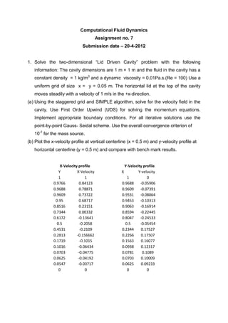
(b) Plot the x-velocity profile at vertical centerline (x = 0.5 m) and y-velocity profile at
horizontal centerline (y = 0.5 m) and compare with bench mark results.
X-Velocity profile Y-Velocity profile
Y X-Velocity X Y-velocity
1 1 1 0
0.9766 0.84123 0.9688 -0.05906
0.9688 0.78871 0.9609 -0.07391
0.9609 0.73722 0.9531 -0.08864
0.95 0.68717 0.9453 -0.10313
0.8516 0.23151 0.9063 -0.16914
0.7344 0.00332 0.8594 -0.22445
0.6172 -0.13641 0.8047 -0.24533
0.5 -0.2058 0.5 -0.05454
0.4531 -0.2109 0.2344 0.17527
0.2813 -0.156662 0.2266 0.17507
0.1719 -0.1015 0.1563 0.16077
0.1016 -0.06434 0.0938 0.12317
0.0703 -0.04775 0.0781 0.1089
0.0625 -0.04192 0.0703 0.10009
0.0547 -0.03717 0.0625 0.09233
0 0 0 0