San Andreas Fault: Fractal of Seismicity

410
Bulletin of the Seismological Society of America, Vol. 94, No. 2, pp. 410–421, April 2004
Fractal Dimension and b-Value on Creeping and Locked Patches of the
San Andreas Fault near Parkfield, California
by Max Wyss, Charles G. Sammis, Robert M. Nadeau, and Stefan Wiemer
Abstract We tested the hypotheses (1) that the fractal dimension, D, of hypo-
centers are different in a locked and a creeping segment of the San Andreas fault
and (2) that the relationship D Ϸ 2b holds approximately, where b is the slope of
the frequency–magnitude relationship. The test area was the 30- to 50-km fault seg-
ment north of Parkfield for which two earthquake catalogs exist: the borehole High
Resolution Seismic Network data, and the U.S. Geological Survey data, which have
a minimum magnitude of completeness of MC 0.4 and MC 1.0–1.2, respectively. The
relative location errors in the two catalogs are estimated as 0.25 km and less than 1
km, respectively. The periods of high-quality data available extend from 1987 to
1998.5 and 1981 to 2000.2, respectively, furnishing 2609 and 3775 events for anal-
ysis, in the two catalogs. In the locked part, 0.5 Ͻ b Ͻ 0.7 and 0.96 Ͻ D Ͻ 1.14,
whereas in the creeping segment, 1.1 Ͻ b Ͻ 1.6 and 1.45 Ͻ D Ͻ 1.72. However,
the spatial distribution of the hypocenters in the creeping segment is not well ap-
proximated by a fractal distribution. We conclude (1) that the frequency–magnitude
distribution as described by b, as well as the fractal dimension (D), are different in
the locked and creeping segments near Parkfield; (2) that the spatial distribution
in the creeping segment is not well approximated by a fractal distribution; and
(3) that the relationship D Ϸ 2b holds in the locked segment, where both parameters
can be measured accurately. Thus, we propose that the heterogeneity of seismogenic
volumes lead to differences in D and b and that these differences, where established
by high-quality data, may furnish clues concerning properties of fault zones.
Introduction
The Parkfield section of the San Andreas fault is located
at the boundary between the creeping section in central Cali-
fornia to the northwest and the locked section north of Los
Angeles to the southeast. It has been the site of a sequence
of six magnitude 6 earthquakes since 1857 (Bakun and
McEvilly, 1984). The last such event occurred in 1966. Fig-
ure 1A shows the epicenters of earthquakes in the magnitude
range ‫2.1מ‬ Ͻ M Ͻ 5 as determined by the High Resolution
Seismic Network (HRSN) operated by the Berkeley Seis-
mological Laboratory and funded by the U.S. Geological
Survey (USGS). It is generally assumed that the fault is
locked in the segment defined by the rectangle in Figure 1
and to the southeast of the seismically active Parkfield seg-
ment. We refer to the hypocentral area of past M 6 main-
shocks as the “Parkfield asperity” (e.g., Lindh and Boore,
1981; Segall and Harris, 1987). The fault surface above and
to the northwest of the asperity is characterized by aseismic
creep that manifests itself by measured fault creep at the
surface. The strongly creeping section northwest of the as-
perity is also characterized by numerous small earthquakes.
The continuous slip along the northwest segment increases
the stress in the asperity in preparation for the next inter-
mediate or large event.
The b-value in the relation log N ‫ס‬ a ‫מ‬ bM varies
strongly in all seismogenic parts of the crust where it has
been mapped on scales from 1 to 30 km (e.g., Ogata et al.,
1991; Wiemer et al., 1998; Wyss et al., 2000; Wyss and
Wiemer, 2000). Wiemer and Wyss (1997) have proposed
that asperities may be characterized by anomalously low b-
values, contrasting especially with the anomalously high b-
values in creeping fault segments. The idea is that b-values
tend to be lower in high-stress asperities because earthquake
ruptures, once nucleated, tend to grow larger in high-stress
environments. This phenomenon has been observed in lab-
oratory experiments (Scholz, 1968), in earthquakes associ-
ated with pumping of fluids (Wyss, 1973), and in under-
ground mines (Urbancic et al., 1992). For the Parkfield
section of the San Andreas fault, b ‫ס‬ 0.5–0.7 in the asperity
and b Ͼ 1.2 in the creeping segment (Amelung and King,
1997; Wiemer and Wyss, 1997).
In this article, we ask whether or not the spatial structure
of the seismicity also reflects this difference between creep-

Fractal Dimension and b-Value on Creeping and Locked Patches of the San Andreas Fault near Parkfield, California 411
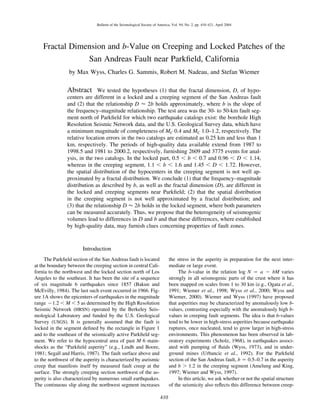
Figure 1. Epicenter maps of earthquakes used. (A) HRSN data, M Ͼ 0.4, for the
period 1987–1998.5; (B) USGS data, M Ͼ 1.0, 1981–2000.2. The polygon shows the
extent of the asperity as defined by Wiemer and Wyss (1997). The stars (arrow) mark
the epicenters of the 1966 fore- and mainshocks. Seismometer stations are shown by
squares.
Table 1
Constants Proposed for Correlating D and b
Model d c d/c Source
Circular, world average 3 1.5 2 Aki (1981)
Elongated, world average 2 1.5 1.33 King (1983)
Parkfield 2.4 1.6 1.5 This article
ing and locked patches. If the spatial structure of seismicity
can be shown to be fractal in a specific volume, then there
is reason to expect the fractal dimension to be correlated with
the b-value in that volume. Aki (1981) pointed out that, if
moment is proportional to fault dimension cubed, then frac-
tal dimension D and b-value should be related as
3
D ‫ס‬ b , (1)
c
where c ഡ 1.5 is the world average scaling constant between
log moment and magnitude (Kanamori and Anderson,
1975). King (1983) generalized equation (1) to
d
D ‫ס‬ b , (2)
c
where d is the scaling exponent between moment and fault
length L (M0 ϰ Ld
). For small earthquakes that grow radially,
d ‫ס‬ 3 as in equation (1) and D ‫ס‬ 2b. For large earthquakes
that span the crust and extend laterally to larger distances,
d ‫ס‬ 2 and D ‫ס‬ 4/3b.
For the Parkfield data set analyzed here, we have spe-
cific information on these constants. Nadeau and Johnson
(1998) observed that the period T of repeating earthquakes
scales as T ϰ . For noninteracting asperities, continuity1/6
M0
of fault displacement requires the same average displace-
ment rate on all asperities, that is, d/T ‫ס‬ constant, indepen-
dent of moment. Hence, d ϰ . Since M0 ‫ס‬ GAd, this1/6
M0
leads to A ϰ or, equivalently, M0 ϰ (L2
)6/5
‫ס‬ L2.4
,5/6
M0
which, by definition, gives d ‫ס‬ 2.4. In addition, an inde-
pendent determination of magnitude and moment for the
events in this study yields log10 M0 ‫ס‬ 1.6M ‫ם‬ 15.8. Thus,
c ‫ס‬ 1.6 for Parkfield events. Hence, based on the Parkfield
data itself, we expect d/c ‫ס‬ 2.4/1.6 ‫ס‬ 1.5. For this model
we assume that no interseismic slip occurs. Other models in
which interseismic slip is allowed can also be constructed
(e.g., Beeler et al., 2001).
The constants proposed for correlating D and b are sum-
marized in Table 1. All of them suggest a positive correla-
tion.
The goals of our study are (1) to test the hypothesis that
D may be different for fault segments with known different
resistance to faulting and (2) to determine the factor corre-
lating D with b along these segments of the San Andreas
fault.
Our study differs from previous attempts to evaluate the
correlation between D and b in several important ways.

412 M. Wyss, C. G. Sammis, R. M. Nadeau, and S. Wiemer
(1) We compared the parameters D and b for fault segments
with known different properties. (2) We used two modern
earthquake catalogs containing accurate hypocenters and
covering the overlapping area with independent recording.
(3) We evaluated important catalog properties, such as the
minimum magnitude of completeness and homogeneity of
reporting as a function of space and time. (4) We paid at-
tention to the hypocenter accuracies, making sure to estimate
D only from a distance range with values larger than the
hypocenter errors.
Data
The primary data set was the catalog derived from the
borehole HRSN data, in which the hypocenter uncertainties
are typically about 0.25 km (Nadeau et al., 1995; Nadeau
and McEvilly, 1999). HRSN locations were determined using
hand-picked P- and S-wave arrivals and a routine (nonrela-
tive) event location method using 3D P and S velocity mod-
els for Parkfield, California (Michelini and McEvilly, 1991;
Nadeau et al., 1994). Root mean square residuals for these
locations are typically 0.02 sec, with horizontal uncertainties
generally one-third the uncertainties in depth. We confirmed
the accuracy of the calculated uncertainties using the empir-
ical method of Nadeau and McEvilly (1997) and the repeat-
ing earthquakes discussed earlier. To verify the reliability of
the results of this accurate, but spatially and temporally re-
stricted, data set, we used the USGS catalog as a secondary
data source with relative hypocenter uncertainties of less
than 1 km. Our estimate of the location error in the USGS
data is based on comparison with relocated hypocenters and
explained in the discussion.
The size of the events reported in the HRSN catalog is
estimated by seismic moment, MO, determined using the
method of Nadeau and Johnson (1998). The HRSN was de-
signed to record microearthquakes on scale to very low mag-
nitudes (ϳ‫1מ‬ Mw), which is possible because of the low
noise environment surrounding the borehole sensors (depths
approximately 200 m). The exceptional noise characteristics
of the borehole seismometers allow for detection of very
small earthquakes; however, the amplification puts limita-
tions on the dynamic range of the data due to the 1980s
technology available at the time of installation of the re-
cording system. This limitation prohibits on-scale recording
of earthquakes larger than about M 1.5–2.0, resulting in
clipped waveforms. While the clipping does not impact the
accuracy of the earthquake locations, it does prohibit accu-
rate determinations of seismic moments for the large events.
Earthquake size for the USGS catalog is primarily based
on coda magnitudes from surface recordings on short-period
sensors in the Northern California Seismograph Network.
Due to the greater noise, the detection threshold of the USGS
network is significantly higher than that of the HRSN and
the accuracy of magnitudes for very small events is dimin-
ished. However, the lower amplification and larger footprint
of the USGS network allows it to record larger events on
scale and to determine their magnitudes accurately.
In order to investigate the relationship between b and D
over a wide magnitude range, and also to compare the results
based on HRSN and USGS data, we convert MO from the
HRSN catalog to magnitudes on the scale used by the USGS.
We then replace the converted magnitudes greater than 1.4
with magnitudes taken from the USGS catalog. The resulting
catalog we call the HRSN catalog hereafter. We have not
introduced additional events in this catalog; we only adjusted
the magnitudes of the larger events. Based on the resulting
frequency–magnitude relation, we conclude that the spliced
catalog is seamless across the splicing magnitude (1.4). This
makes it possible to map the distribution of b-values on a
fine scale (Figs. 2 and 3).
The moment-to-magnitude conversion used was
log(MO) ‫ס‬ 1.6*M ‫ם‬ 15.8 (MO in dyne centimeters and log
to base 10). The two constants in this equation were deter-
mined empirically by a least-squares fit, using a set of 386
repeating earthquakes common to the HRSN and USGS cat-
alogs and located within the smaller footprint of the HRSN.
We used repeating earthquakes, events having essentiallythe
same hypocenter and virtually identical seismograms, be-
cause both relative and absolute estimates of their locations
and seismic moments can be much better constrained by
cross-correlation and spectral ratio processing and by aver-
aging over redundancies (Nadeau and McEvilly, 1997; Na-
deau and Johnson, 1998). These events were from the over-
lap of the two catalogs, which covers the range 0.60 Յ M
Յ 1.70 on the USGS scale.
As a next step, we assessed the quality and the extent
of usefulness of the HRSN catalog in space, time, and mag-
nitude band. (1) Using the GENAS algorithm (Habermann,
1983), implemented in the ZMAP program (Wiemer, 2001),
we found that the catalog is homogeneous in reporting earth-
quakes from 1987 through the end of the data in 1998.5.
There was no evidence of any change in the scale to measure
earthquake size. (2) The spatial extent of the high-quality
catalog was estimated by mapping the minimum magnitude
of completeness, Mc. North of 36.03Њ and south of 35.83Њ,
the Mc increased rapidly from the average value of Mc 0.4
within the well-covered segment of the fault. In the critical
segments of the asperity and the creeping sections neigh-
boring it (35.91Њ Ͻ lat Ͻ 36.01Њ), the Mc is uniformly equal
to 0.4. The only segment with inferior resolution (Mc 0.7) is
located south of the asperity (35.87Њ Ͻ lat Ͻ 35.9Њ). This
segment does not play an important role in our analysis. The
critical comparison of properties is derived from the asperity
and creeping segments between 35.91Њ and 36.01Њ latitude,
which are covered with uniform quality.
Given the various restrictions explained earlier, the
HRSN data consist of the events with M Ն 0.4 in the latitude
range shown in Figure 1A, during the period 1987–1998.5,
totaling 2609 events.
The advantages of the USGS data are that they cover a
longer segment of the fault and that they include larger num-

Figure 2. Cross-section map of b-values, using the 180 events nearest nodes spaced
0.3 km apart, provided they occurred within 5 km of the node. White areas contain
nodes that do not have 180 events within 5 km. The circles and polygons define the
volumes selected for the frequency–magnitude distribution plots in Figure 3A,B, re-
spectively. Stars mark hypocenters of the 1966 fore- and mainshocks. Both occurred
in what is generally known as the Middle Mountain asperity.
bers of earthquakes, both because of the greater spatial cov-
erage and the longer observation period of high-quality data
(1981–2000.2, the end of the data at the time of this analy-
sis). The Mc for these data in the study area was mapped as
1.2 (Wiemer and Wyss, 2000). The spatial limits for the
USGS data (Fig. 1B) were not selected on the basis of Mc,
because that value is uniform in a fairly large area of central
California. In this case, the study segment of the fault was
extended such that we doubled the information on the creep-
ing segment to the north and on the locked segment to the
south, approximately (Fig. 1B).
The extent of the Parkfield asperity, as defined by the
anomaly of local recurrence time (Wiemer and Wyss, 1997),
is about 10 km long and is shown as the rectangle containing
the epicenters of the 1966 main- and foreshock (stars) in
Figure 1. Selecting the data within it as one of the data sets
for our test leaves a segment of equal length in the creeping
segment north of it for comparison, using the HRSN data
(Fig. 1A). To demonstrate that any contrast in D between
locked and creeping segments does not depend on the exact
selection of the test section, we extended the data in the
USGS set to about 20 km north and 20 km south of the
asperity (Fig. 1B).
Measuring the b-Value
The b-values were measured by the maximum likeli-
hood method (Aki, 1965; Bender, 1983). However, all es-
timates were also performed using the weighted least-
squares method (Shi and Bolt, 1982) to ensure that the
method did not change the result by more than 0.1 units. The
formal errors in the b-value fits were typically less than, but
close to, 0.1 units. Also, we used several definitions of the
creeping and the asperity segments, in order to make sure
that the contrast in the parameters does not depend on the
exact selection criteria.
The volumes for the b-value analyses were defined as
follows: The extent of the asperity segment (Fig. 1) was first
estimated based on the results of Wiemer and Wyss (1997),
who used the USGS data for the period 1981–1996. The
creeping segment was taken to be the rest of the data to the
northwest of the polygon in Figure 1, for the respective data
sets. The comparison between the b-value for the asperity
and creeping segment thus defined is given in Figure 3C for
the HRSN data and Figure 3F for the USGS data set.
In order to define the asperity more precisely, the b-
value was mapped in cross section (Fig. 2) based on the
HRSN data. Circles containing equal numbers of events
(N ‫ס‬ 180) were selected in the heart of the asperity and
creeping segments, as indicated on Figure 2. We chose N ‫ס‬
180 because this way the sizes of the sampled volumes range
from 1 to 5 km, approximately. Smaller and larger volumes
than these are not desirable for mapping b-value contrasts in
a stable way. The b-values for the asperity and creeping
segments as defined by these circles are compared in Figure
3A,D for the HRSN and the USGS data, respectively. Radii
of the corresponding circles in the USGS cross section (not
shown) were 4.5 and 3.0 km. Finally, somewhat larger poly-
gons were chosen to represent the asperity and creeping sec-
tions in the cross section for both data sets, in order to also

Figure 3. Frequency–magnitude distributions comparing samples from the asperity
and creeping fault segments (squares mark data from the asperity, circles from the
creeping section). (A) HRSN data from the volumes defined by circles in Figure 2. (B)
HRSN data using polygons in Figure 2 to separate the asperity and creeping segments.
(C) HRSN data from the area within the polygon in Figure 1A compared to all the data
northwest of it. (D) USGS data from circles in asperity and creeping sections having
4.5 and 3 km in radii, respectively. (E) USGS data based on polygons created in cross
section. (F) USGS data from the polygon in Figure 2B, compared to the data north of
it. The value p in the top right corner of each frame gives the probability that the two
samples come from the same population (Utsu, 1992).
take into account that asperity and creeping sections defined
by Wiemer and Wyss (1997) were located below and above
about 6 km depth, respectively. The polygons chosen for the
HRSN data are shown in Figure 2, and in Figure 3B b-value
for these two polygons are compared. The USGS data for the
same polygons are compared in Figure 3E. Utsu’s (1992)
test for estimating the significance of differences between
samples is applicable because the limits of the samples in
space, time, and magnitude band were defined by Wiemer
and Wyss (1997), independent of the b-values of each sam-
ple in this study.
The frequency–magnitude distributions for all samples
from creeping sections differ strongly from those of the
locked segments (Fig. 3). Visual inspection of this figure
confirms the result that the probability that these pairs of
samples come from the same population is vanishingly
small, as estimated by Utsu’s (1992) test. The average dif-
ference in b is 0.67 for the results summarized in Table 2.
The difference is largest for the circles centered on the as-
perity and on the creeping segment.
Measuring the Fractal Dimension
To determine the fractal dimension, we use the two-
point correlation dimension defined as (Schroeder, 1991)
logC(r)
D ‫ס‬ lim , (3)2
logrr→0

Table 2
Comparison of b-Values between Asperity and Creeping Sections
HRSN
Section Circle
USGS
Section Circle
HRSN
Section Polygon
USGS
Section Polygon
HRSN
Map View
USGS
Map View
Asperity 0.45 0.50 0.61 0.64 0.69 0.69
Creep 1.60 1.90 1.03 1.09 0.94 1.08
where C(r) is the pair correlation function. It is defined as
N(s Յ r)
C(r) ‫ס‬ , (4)2
Ntot
where N(s Յ r) is the number of point pairs whose Euclidean
separation distance, s, is less than r, and Ntot is the total
number of points. For deterministic monofractals, D2 ‫ס‬ D0.
Unlike b-value, where the spatial resolution of the map-
ping is limited by the number of events, the spatial resolution
of fractal dimension maps is limited by the location accu-
racy. For the Parkfield borehole array, the average spatial
resolution is 150–250 m. Since a meaningful fractal analysis
requires at least 1 order of magnitude range of lengths, the
minimum patch size required for fractal analysis is about
2 km. The asperity and creeping regions are each only about
10 km long (Fig. 2), so we did not attempt to subdivide these
regions for the fractal analysis. The uncertainty of D is com-
puted using the aleatory uncertainty on the fit only, not tak-
ing into account uncertainty in hypocenter locations or in the
estimate of the fitting range. Consequently, the uncertainties
given by us tend to be small. Uncertainties that also consider
epistemic contributions would be larger; however, they rep-
resent a mixture of various contributions to uncertainty and
depend on assumptions on hypocenter uncertainties and
range estimates. We therefore feel that it is more appropriate
to list the formal errors of the fit only. Because the differ-
ences in D that we discuss in this article are all highly sig-
nificant, they cannot be explained by uncertainties in the
estimation of D.
Results of the fractal analysis are shown in Figure 4 and
summarized in Table 3. The section of each curve that is fit
by a straight line is not preselected. Only the approximately
straight section of the curve is used. Data from distances
shorter than the hypocentral location errors (0.25 km for
HRSN and 1 km for USGS) are not used. For shorter distances
than these, the slope approaches 2, the expected result for
random locations on a plane.
In the asperity region, the fractal dimension is near 1.
This is compatible with the analysis of Sammis et al. (1999),
who found D ‫ס‬ 1 over distances ranging from 10 m to 20
km. They were able to measure over a wider range of sep-
arations by only using the best located events as centers of
the correlation analysis. In the creeping section, the fractal
dimension is significantly higher, 1.45–1.72. Careful ex-
amination of Figure 4A,C suggests that the distribution may
not be fractal in the creeping section since the correlation
integral shows continuous curvature for R Ͼ 200 m. This
contrasts with the asperity region where the distribution
clearly shows a flat segment.
Discussion
In the area of the asperity, the b-value is low (0.5 Ͻ b
Ͻ 0.7, Table 2) as is the fractal dimension (0.96 Ͻ D Ͻ
1.14, Table 3). In the creeping segment to the north, the b-
value is significantly higher (1.1 Ͻ b Ͻ 1.6, Table 2), but
the spatial distribution of hypocenters is not strictly fractal
since the plot of logN versus logR in Figure 4 shows cur-
vature over the range of significant distances (R Ͼ 200m).
Nevertheless, the approximate slope for R Ͼ 200m corre-
sponds to 1.45 Ͻ D Ͻ 1.72 (Table 3), significantly larger
than that in the locked segment. Hence, our results show a
positive correlation between D and b (Fig. 5).
Errors in Hypocenter Locations
The accuracy of hypocenter locations is a crucial issue,
if one attempts to estimate the fractal dimension of earth-
quakes from the distances separating them. Several authors
have studied the influence of geometry and other limits of
the data on the estimate of D (e.g., Nerenberg and Essex,
1990; De Luca et al., 1999), but few have considered the
size of the hypocenter errors and their influence (Kagan and
Knopoff, 1980; Eneva, 1996). As far as we can find, none
of the authors attempting to correlate b and D have paid
specific attention to this problem.
Interevent distances smaller than the error of hypocenter
locations are meaningless. Thus, fractal dimensions can only
be estimated from a range of distances that is entirely larger
than the errors. If Xerr and Zerr are the horizontal and vertical
errors, respectively, and if we assume that Zerr Ͼ Xerr, then
the radii for estimating D must be R Ͼ Zerr. For the sake of
keeping our argument simple, we assume that the minimum
radius that may be used for estimating D is approximately
Rmin ‫ס‬ Zerr. Although we do not know the distribution of
the errors around the true location, it is clear that the errors
tend to have the effect of randomizing the distribution within
volumes smaller then the mean error. Thus, the data in a
range R Ͻ Zerr are expected to yield large values for D,
approaching 3. Therefore, we expect a result as shown in
Figure 6, with a steep slope at the lower end. We checked
this phenomenon in several earthquake catalogs (Coso,
southern California, Bosai, Tohoku, Alaska) and found that

Figure 4. Correlation integrals versus interevent distance for different fault seg-
ments and data sets. (A), (B), and (E) are for HRSN data; (C), (D), and (F) are for USGS
data. The resulting fractal dimensions, D, are indicated in each frame. The distance
ranges for the straight-line ﬁts are given as r in each frame. “Asperity” refers to the
data from the polygons shown in Figure 1, “creep” refers to the data northwest of the
polygon, “south” signiﬁes the data southeast of the polygon in Figure 1B, and “asperity
‫ם‬ south” means the data within plus southeast of the polygon in Figure 1A. Dashed
lines with a slope of 1, as seen in the asperity data, illustrate the difference of the
observed data from the creeping section.

Table 3
Fractal Correlation Dimension of Hypocenters
Asperity Asperity ‫ם‬ South South Creep
HRSN 1.14 ‫ע‬ 0.02 1.13 ‫ע‬ 0.03 1.72 ‫ע‬ 0.03
USGS 0.96 ‫ע‬ 0.03 1.10 ‫ע‬ 0.02 1.45 ‫ע‬ 0.04
Figure 5. Fractal correlation dimension, D, as a
function of b-value. The parameter of the solid lines
is the theoretically expected factor (d/c) governing the
relationship between the two parameters. The two rec-
tangles show the range of values observed in the two
fault segments.
Figure 6. Schematic plot of a correlation integral
as a function of radius over a range of distances from
smaller than to larger than Rmin, which equals the hy-
pocenter error.
in all cases the slope at distances shorter than Zerr was ap-
proximately D ‫ס‬ 2.5, whereas above Zerr ‫ס‬ Rmin the slope
varied between 1 and 1.5. Figure 6 is similar to the plot
shown by Volant and Grasso (1994) in their figure 4, but
they interpreted both slopes as reflecting real distribution
characteristics. We interpret the break in slope as due to the
location error.
In the literature comparing b with D, two types of cat-
alogs are used: (1) teleseismic and offshore catalogs with
relatively large errors and (2) local catalogs with smaller
errors. We propose that in category 1, Rmin Ն 10 km, and in
category 2, Rmin Ն 1 km, in the best cases. For rock bursts
in mines, the errors are far smaller, as for example 8–15 m,
as reported by Eneva (1996). However, in most earthquake
catalogs, the errors are substantially larger than those we
propose as lower limits. Our estimates of typical errors in
catalogs come from comparisons of the scatter of hypocen-
ters of relocated events with the scatter in the original cat-
alog, as explained later.
Generally, network operators producing catalogs of the
second type are aware that hypocentral errors measure a few
kilometers. However, often the size of the errors are unex-
pectedly large, as in the case of the New Madrid seismic
zone, where Chiu et al. (1992) achieved spectacular im-
provements of the locations by a new method of locating
them. In cross sections, clouds of hypocenters more than
10 km wide contracted to zones less than 2 km thick. Thus,
in New Madrid, the errors in depth were at least Zerr ‫ס‬ ‫4ע‬
km, in spite of coverage by a relatively dense local seis-
mograph network. One may argue that this was a special
case, because a change of phase interpretation was discov-
ered. Thus, we base our estimate of errors on the reduction
in the scatter of relocated earthquakes in Hawaii (Gillard et
al., 1996) and California (Waldhauser and Ellsworth, 2000).
In Hawaii, shallow earthquakes in a volume of about 5-km
dimensions were registered by a network with about 5-km
station separation, including four three-component stations
within approximately 6 km. The original apparent width of
the seismically active zone was 0.8 km, and the depth dis-
tribution covered 2 km. After relocation by a precise tech-
nique, this cloud of hypocenters contracted to less than 0.1-
km extent in both vertical and horizontal directions (figure
2 of Gillard et al. [1996]). Thus, we conclude that the errors
in the standard catalog of Hawaiian earthquakes are approx-
imately Zerr ‫ס‬ ‫0.1ע‬ km and Xerr ‫ס‬ ‫4.0ע‬ km. In California
the interstation distances are about 10 km. In this area, the
relocations of Waldhauser and Ellsworth (2000) reduced the
original scatter of ‫5.0ע‬ km in both the X and the Z directions
to less than ‫1.0ע‬ km. Thus, we conclude that in one of the
most carefully monitored parts of California, the hypocentral
errors in recent years were approximately ‫5.0ע‬ km. Because
these two networks are among the very densest and most
carefully operated, the errors in local catalogs in general
have to be assumed to be larger than 1 km, and hence we
propose that the correlation integral makes sense only for
R(local network) Ն 1 km. None of the work known to us

that correlates b with D derived the latter parameter from a
range of R clearly larger than the location error.
Based on this criterion, we interpret figure 4 of Volant
and Grasso (1994) as demonstrating that Rmin ‫ס‬ Zerr ‫ס‬ 0.5
km in their catalog. Since their seismograph network con-
tained only nine stations in an area of 15-km dimensions,
including only one three-component station, it is expected
to furnish location accuracies inferior to the Hawaiian net-
work. Thus, it is very unlikely that their value for D esti-
mated for their range R Ͻ 0.5 km is meaningful. The same
is true for the work by Guo and Ogata (1995, 1997). In about
a quarter of their 34 cases, their estimate of D was based on
a range of R Ͻ 2 km, with the lower bound usually between
0.2 and 0.4 km. The break in slope at 2 km in their figure 5
suggests that Rmin ‫ס‬ 2 km, in their cases of earthquakes
below the land mass. Approximately half of their study areas
are located offshore, some far offshore. The recent catalogs
of the best networks in Japan show scatter of 100 km for Z
in offshore areas. In other words, the depth is not known
offshore, and the epicentral errors must be assumed to be
large also. Near land, the errors are not quite as large, but it
is unrealistic to assume that the errors would be as little as
0.5–2 km, as proposed by Guo and Ogata (1997).
The range of observations of D in two articles on geo-
thermal areas are 0.08 Ͻ R Ͻ 0.45 km (Henderson et al.,
1999) and 0.4 Ͻ R Ͻ 1 km (Barton et al., 1999). The ac-
curacies of hypocenter locations implied by these analyses
are usually only achieved by special efforts, such as those
of Gillard et al. (1996) or Waldhauser and Ellsworth (2000).
They are not likely to be realized in the catalogs these au-
thors used.
For teleseismic locations, catalogs of type 1, the differ-
ence in epicenters compared to locations based on local net-
works is typically 15 km for recent years. This has been
verified, for example, by comparing aftershock locations ob-
tained by a temporary network with teleseismic locations of
the same events in Sakhalin (Wyss et al., 2004). For shallow
earthquakes, the teleseismic depth is often uncertain to Zerr
(tele) ‫ס‬ ‫03ע‬ km, because depth phases can only be read
for events deeper than about 60 km. In island arcs, the sys-
tematic errors can change rapidly from about 50 km out-
board of the arc (Engdahl et al., 1982; Papadopoulos et al.,
1988) to the usual 10- to 20-km inboard. Thus, even rela-
tively modern teleseismic catalogs contain Xerr k 10 km in
off shore areas, and old catalogs starting in 1900 (used by
Oencel et al. [1996]) or 1923 (used by Hirata [1989]) contain
location errors that are typically several tens of kilometers.
Such catalogs cannot be used for estimating D.
We conclude that we could not find a paper correlating
b and D in which the estimate of D was derived from a range
of distances above Rmin, labeled “meaningful slope” in Fig-
ure 6. Thus, we see the need of a generation of careful anal-
yses of b versus D, based on data from high-quality earth-
quake catalogs entirely in the range above Rmin.
Reporting Heterogeneity as a Function of Time
In addition to inaccurate locations, reporting heteroge-
neities as a function of time can lead to artificial variations
in b-values (Zuniga and Wyss, 1995; Zuniga and Wiemer,
1999) and, over long periods, hypocenter errors also change.
Therefore, conclusions about differences in b or D derived
by comparing data from different periods, as done by Okubo
and Aki [1987] and Henderson et al. [1992], are unreliable,
unless a detailed analysis of the temporal stability of the
catalog has shown that magnitude scale and hypocenter ac-
curacy have not changed.
We believe that only the most reliable data sets can be
used to establish the relationship between D and b and that
many investigators underestimate the degree of heteroge-
neity of earthquake catalogs. We judge the catalogs we used
as relatively homogeneous as a function of time and space,
based on the following observations. (1) The HRSN catalog
covers a short period and a small area, and the station net-
work was constant. (2) The minimum magnitude of com-
pleteness is constant with time in both catalogs. (3) The b-
values are approximately constant with time in both
catalogs. (4) Features that could be interpreted as due to
artificial reporting rate changes as a function of time are not
present in the HRSN catalog. The USGS catalog contains
such features; thus an analysis of D as a function of time
might be questionable, and we do not attempt it. We have
no evidence about possible changes of the accuracy of hypo-
centers as a function of time and assume that there were only
minor changes because the network configuration did not
change significantly in either network. Thus, we believe that
the two data sets used are some of the very best available
from the point of view of detail and stability.
Comparison of Observed with Theoretical
Relationships between b and D
Figure 5 shows that equation (2) with the value of
d/c ‫ס‬ 2 leads to a good fit for data in the asperity region.
However, for the data in the creeping section the preferred
value is approximately d/c ‫ס‬ 1.3. In Figure 5, d/c ‫ס‬ 1.5
intersects both data fields, the one for the asperity and for
the creeping section, although just barely. This value of
d/c ‫ס‬ 1.5, selected by the combined data sets, is what we
expect, based on other information (Nadeau and Johnson,
1998) available for the Parkfield area (Table 1).
These observations raise a number of fundamental ques-
tions. First, why is the spatial distribution better described
by a power law at the asperity than in the creeping section
(Fig. 4), even though both areas satisfy the Gutenberg–
Richter relation equally well (Fig. 3)? The answer may lie
in the fact that King’s (1983) proposed geometrical origin
of b-value does not require a spatially fractal distribution of
faults. It is simply the mapping from a power-law distribu-
tion of rupture sizes to the frequency–magnitude relation-
ship, assuming a logarithmic scaling between magnitude and

moment, and a power-law scaling between moment and fault
length. There is, however, no requirement that the power-
law distribution of ruptures also form a spatial fractal. King
(1983) envisioned the formation of a spatially fractal net-
work of faults as a way to accommodate geometrical incom-
patibilities, like bends and jogs of the fault plane, using only
brittle deformation. However, on a creeping fault, such geo-
metrical constraints do not apply. This is especially true for
the creeping section at Parkfield, where the earthquakes oc-
cur on stuck asperities that only make up a small fraction of
the fault surface (Nadeau and Johnson, 1998).
For example, imagine populating a uniform grid with a
power-law distribution of asperities as follows: one asperity
of radius r, n asperities of radius r/m, n2
of radius r/m2
, and
so on. King’s relation, D ‫ס‬ (d/c)b, would still be valid
where D ‫ס‬ logn/logm. However, the spatial correlation di-
mension would be D2 ‫ס‬ 2, reflecting the uniform spatial
distribution. Of course, these asperities do not tile the fault
surface, but this is not required on a creeping fault plane.
The question is, why should an ensemble of isolated asper-
ities have a power-law size distribution?
One possible explanation is that the locked asperities
physically correspond to blocks of very strong rock (knock-
ers), commonly observed in Franciscan terrains (Coleman
and Lanphere, 1971; Karig, 1979). Creep on the central sec-
tion of the San Andreas fault is correlated with Franciscan
wall rock and is believed to be due to the mechanical prop-
erties of serpentinite and other hydrous phases (Allen, 1968).
Knockers are isolated blocks of very strong, high-grade
metamorphic rocks and eclogites within the weak trench de-
posits. Coleman and Lanphere (1971) pointed out that field
relationships indicate the blocks are closely associated with
serpentine and that they occupy disturbed zones that may be
related to faulting. The blocks range in size from 1.5 to
300 m in diameter to a few larger masses, as much as 11 km
long and 3 km wide. The shape of individual blocks is el-
lipsoidal. Some are nearly spherical, while others are prolate
or oblate ellipsoids. This led Brune and Anooshehpoor
(1997) to propose that these blocks may act as rotor bearings
in the fault zone that reduce friction. However, the outer
surfaces of the blocks are commonly grooved and striated,
implying slip at their surfaces. We suggest the alternative
hypothesis that the blocks act as pinning points on the oth-
erwise creeping fault plane and that they fail catastrophically
as small earthquakes.
If the knockers in the creeping segment are fragmented
by shear flow, then they might be expected to have a power-
law distribution of fragment sizes, even if the individual
fragments are subsequently spread apart by flow in the fault
zone and no longer have a fractal structure in space. The
power-law distribution of particles produced by the in situ
fragmentation of 3D knockers corresponds to D ‫ס‬ 2.6
(Sammis et al., 1987). This interpretation is consistent with
d/c ‫ס‬ 2, but not with d/c ‫ס‬ 1.5, which fits both observa-
tions. Perhaps fragmentation of knockers caught in a fault
zone produces a lower fractal dimension than the D ‫ס‬ 2.6
observed for the formation of fault gouge from brittle rock.
A second question is, why are b and D so low in the
asperity? A simple explanation of the observation that D Ϸ
1 is that the hypocenters are arranged in linear structures.
Linear streaks of hypocenters have been observed by Rubin
et al. (1999) at the north end of the creeping segment near
San Juan Bautista and have been postulated by Sammis and
Rice (2001) to represent boundaries between creeping and
locked fault patches. If D ‫ס‬ 1, the condition of uniform
displacement on the line requires b ‫ס‬ 0.5 according to
King’s argument. However, high-resolution locations by Na-
deau and McEvilly (1997) have not revealed pronounced
lineations at Parkfield. Although Sammis et al. (1999) ob-
served D Ϸ 1 for their locations over 4 orders of magnitude
in event separation, the structure near Parkfield seems to be
more of a discrete nested hierarchy of clusters within clus-
ters, morphologically similar to a 2D Cantor Dust. One pos-
sibility is that this nested hierarchy corresponds to a sequen-
tial breakup of knockers in the shear flow where fragments
in a large cluster separate and are, in turn, fragmented into
smaller clusters. Perhaps, at the northern end of the creeping
segment, the knocker fragments have, for some reason, been
strung out into long streaks by the flow. A more quantitative
assessment of such a mechanism requires a better under-
standing of how hard inclusion fragments are and how they
are dispersed in a shear flow.
Conclusions
We conclude that the creeping portion of the San An-
dreas fault near Parkfield has higher b- and D-values than
the locked portion. This result is robust for the following
reasons. (1) The observation is made in two independent data
sets. (2) The observation remains the same, independent of
the exact definition of the volumes used for sampling.
(3) The difference is substantial.
It may be that the relationship between b and D is dif-
ferent in the two fault segments: D ഡ 2b and D ഡ b in the
locked and creeping segments, respectively. However, one
might alternatively argue that D ഡ 1.5b can marginally sat-
isfy the data from both fault segments.
We suggest that a new effort should be made to deter-
mine D for earthquake distributions because not enough at-
tention has been paid to the randomizing effect that hypo-
center errors introduce. In the estimates of D known to us,
the underestimates of the hypocenter errors render the results
suspect.
We conclude that currently there remain many open
questions about the details of the makeup of fault zones and
that careful studies of the relationship between fractal di-
mensions and b-value are likely to furnish important con-
straints for fault models.

Acknowledgments
Part of this work was carried out while M. W. was employed by the
Geophysical Institute of the University of Alaska, Fairbanks, and it was
partially supported by the SCEC project. Additional support came from the
U.S. Geological Survey through Award Number 03HQGR0065 and by the
National Science Foundation through Award Number 9814605. Partial pro-
cessing of the data was done at the University of California’s Berkeley
Seismological Laboratory and at the Center for Computational Seismology
(CCS) at Lawrence Berkeley National Laboratory.
References
Aki, K. (1965). Maximum likelihood estimate of b in the formula log
N ‫ס‬ a ‫מ‬ b M and its confidence limits, Bull. Earthquake Res. Inst.
43, 237–239.
Aki, K. (1981). A probabilitstic synthesis of precursory phenomena, in
Earthquake Prediction: An International Review, D. W. Simpson and
P. G. Richards (Editors), American Geophysical Union, Washington,
D.C., 566–574.
Allen, C. R. (1968). The tectonic environments of seismically active and
inactive areas along the San Andreas fault systems, in Conf. of Geo-
logical Problems of San Andreas Fault System, W. R. Dickenson and
A. Grantz (Editors), Stanford U Publications, Stanford, California.
Amelung, F., and G. King (1997). Earthquake scaling laws for creeping
and non-creeping faults, Geophys. Res. Lett. 24, 507–510.
Bakun, W. H., and T. V. McEvilly (1984). Recurrence models and Park-
field, California, earthquakes, J. Geophys. Res. 89, 3051–3058.
Barton, D. J., G. R. Foulger, J. R. Henderson, and B. R. Julian (1999).
Frequency–magnitude statistics and spatial correlation dimensions of
earthquakes at Long Valley caldera, California, Geophys. J. Int. 138,
563–570.
Beeler, N. M., D. A. Lockner, and S. H. Hickman (2001). A simple stick-
slip and creep-slip model for repeating earthquakes and its implication
for microearthquakes at Parkfield, Bull. Seism. Soc. Am. 91, 1797–
1804.
Bender, B. (1983). Maximum likelihood estimation of b-values for mag-
nitude grouped data, Bull. Seism. Soc. Am. 73, 831–851.
Brune, J. N., and A. Anooshehpoor (1997). Frictional resistance of a fault
zone with strong rotors, Geophys. Res. Lett. 24, 2071–2074.
Chiu, J. M., A. C. Johnston, and Y. T. Yang (1992). Imaging the active
faults of the central New Madrid seismic zone using PANDA array
data, Seism. Res. Lett. 63, 375–393.
Coleman, R. G., and M. A. Lanphere (1971). Distribution and age of high-
grade blueschists, associated ecolgites, and amphiboles from Oregon
and California, Geol. Soc. Am. Bull. 82, 2397–2412.
De Luca, L., S. Lasocki, D. Luzio, and M. Vitale (1999). Fractal dimension
confidence interval estimation of epicentral distributions, Ann. Geofis.
42, 911–925.
Eneva, M. (1996). Effect of limited data sets in evaluating the scaling prop-
erties of spatially distributed data: an example from mining-induced
seismic activity, Geophys. J. Int. 124, 773–786.
Engdahl, E. R., J. W. Dewey, and K. Fujita (1982). Earthquake location in
island arcs, Phys. Earth Planet. Interiors 30, 145–156.
Gillard, D., A. M. Rubin, and P. Okubo (1996). Highly concentrated seis-
micity caused by deformation of Kilauea’s deep magma system, Na-
ture 384, 343–346.
Guo, Z., and Y. Ogata (1995). Correlation between characteristic parame-
ters of aftershock distribution in time, space, and magnitude, Geophys.
Res. Lett. 22, 993–996.
Guo, Z. Q., and Y. Ogata (1997). Statistical relations between the param-
eters of aftershocks in time, space, and magnitude, J. Geophys. Res.
102, 2857–2873.
Habermann, R. E. (1983). Teleseismic detection in the Aleutian Island arc,
J. Geophys. Res. 88, 5056–5064.
Henderson, J., D. Barton, and G. Foulger (1999). Fractal clustering of in-
duced seismicity in the Geysers geothermal area, California, Geophys.
J. Int. 139, 317–324.
Henderson, J. R., I. G. Main, P. G. Meredith, and P. R. Sammonds (1992).
The evolution of seismicity at Parkfield, California: observation, ex-
periment, and a fracture-mechanical interpretation, J. Struct. Geol. 14,
905–913.
Hirata, T. (1989). A correlation of b-value and fractal dimension of earth-
quakes, J. Geophys. Res. 94, 7507–7514.
Kagan, Y. Y., and L. Knopoff (1980). Spatial distribution of earthquakes:
the two-point correlation function, Geophys. J. R. Astr. Soc. 62, 303–
320.
Kanamori, H., and D. L. Anderson (1975). Theoretical basis of some em-
pirical relations in seismology, Bull. Seism. Soc. Am. 65, 1073–1095.
Karig, D. E. (1979). Material transport within accretionary prisms and the
“knocker” problem, J. Geol. 88, 27–39.
King, G. C. P. (1983). The accommodation of large strains in the upper
lithosphere of the Earth and other solids by self-similar fault systems:
the geometrical origin of b-value, Pure Appl. Geophys. 121, 761–815.
Lindh, A. G., and D. M. Boore (1981). Control of rupture by fault geometry
during the 1966 Parkfield earthquake Bull. Seism. Soc. Am. 71, 95–
116.
Michelini, A., and T. V. McEvilly (1991). Seismological studies at Park-
field, part I: Simultaneous inversion for velocity structure and hypo-
centers using B-splines parameterization, Bull. Seism. Soc. Am. 81,
524–552.
Nadeau, R. M., and L. R. Johnson (1998). Seismological studies at Park-
field, part IV: Moment release rates and estimates of source param-
eters for small repeating earthquakes, Bull. Seism. Soc. Am. 88, 790–
814.
Nadeau, R. M., and T. V. McEvilly (1997). Characteristic microearthquakes
sequences as fault-zone drilling targets, Bull. Seism. Soc. Am. 87,
1463–1472.
Nadeau, R. M., and T. V. McEvilly (1999). Fault slip rates at depth from
recurrence intervals of repeating microearthquakes, Science 285, 718–
721.
Nadeau, R., M. Antolik, P. A. Johnson, W. Foxall, and T. V. McEvilly
(1994). Seismological studies at Parkfield, part III: Microearthquake
clusters in the study of fault-zone dynamics, Bull. Seism. Soc. Am.
84, 247–263.
Nadeau, R., W. Foxall, and T. V. McEvilly (1995). Clustering and periodic
recurrence of microearthquakes on the San Andreas fault, Science
267, 503–507.
Nerenberg, M. A. H., and C. Essex (1990). Correlation dimension and
systematic geometric effects, Phys. Rev. A 42, 7065–7074.
Oencel, A. O., I. Main, O. Alptekin, and P. Cowie (1996). Spatial variations
of the fractal properties of seismicity in the Anatolian fault zones,
Tectonophysics 257, 189–202.
Ogata, Y., M. Imoto, and K. Katsura (1991). 3-D spatial variation of b-
values of magnitude–frequency distribution beneath the Kanto dis-
trict, Japan, Geophys. J. Int. 104, 135–146.
Okubo, P. G., and K. Aki (1987). Fractal geometry of the San Andreas
fault system, J. Geophys. Res. 92, 345–355.
Papadopoulos, T., D. L. Schmerge, and M. Wyss (1988). Earthquake lo-
cations in the western Hellenic arc relative to the plate boundary, Bull.
Seism. Soc. Am. 78, 1222–1231.
Rubin, A. M., D. Gillard, and J. L. Got (1999). Streaks of microearthquakes
along creeping faults, Nature 400, 635–641.
Sammis, C. G., and J. R. Rice (2001). Repeating earthquakes as low-stress-
drop events at a border between locked and creeping fault, Bull.
Seism. Soc. Am. 91, 532–537.
Sammis, C. G., G. King, and R. Biegel (1987). The kinematics of gouge
deformation, Pure Appl. Geophys. 125, 777–812.
Sammis, C. G., R. M. Nadeau, and L. R. Johnson (1999). How strong is
an asperity? J. Geophys. Res. 104, 10,609–10,619.
Scholz, C. H. (1968). The frequency–magnitude relation of microfracturing
in rock and its relation to earthquakes, Bull. Seism. Soc. Am. 58, 399–
415.

Schroeder, M. (1991). Fractals, Chaos, Power Laws, Freeman, San Fran-
cisco.
Segall, P., and R. Harris (1987). Earthquake deformation cycle on the San
Andreas fault near Parkfield, California, J. Geophys. Res. 92, 10,511–
10,525.
Shi, Y., and B. A. Bolt (1982). The standard error of the magnitude–
frequency b value, Bull. Seism. Soc. Am. 72, 1677–1687.
Urbancic, T. I., C. I. Trifu, J. M. Long, and R. P. Young (1992). Space-
time correlations of b-values with stress release, Pure Appl. Geophys.
139, 449–462.
Utsu, T. (1992). On seismicity, in Report of the Joint Research Institute for
Statistical Mathematics, Institute for Statistical Mathematics, Tokyo,
139–157.
Volant, P., and J. R. Grasso (1994). The finite extension of fractal geometry
and power law distribution, J. Geophys. Res. 99, 21,879–21,890.
Waldhauser, F., and W. L. Ellsworth (2000). A double-difference earth-
quake location algorithm: method and application to the northern
Hayward fault, California, Bull. Seism. Soc. Am. 90, 1353–1368.
Wiemer, S. (2001). A software package to analyze seismicity: ZMAP, Seism.
Res. Lett. 373–382.
Wiemer, S., and M. Wyss (1997). Mapping the frequency–magnitude dis-
tribution in asperities: an improved technique to calculate recurrence
times? J. Geophys. Res. 102, 15,115–15,128.
Wiemer, S., and M. Wyss (2000). Minimum magnitude of complete re-
porting in earthquake catalogs: examples from Alaska, the western
United States, and Japan, Bull. Seism. Soc. Am. 90, 859–869.
Wiemer, S., S. R. McNutt, and M. Wyss (1998). Temporal and three-
dimensional spatial analysis of the frequency–magnitude distribution
near Long Valley caldera, California, Geophys. J. Int. 134, 409–421.
Wyss, M. (1973). Towards a physical understanding of the earthquake fre-
quency distribution, Geophys. J. R. Astr. Soc. 31, 341–359.
Wyss, M., and S. Wiemer (2000). Change in the probability for earthquakes
in southern California due to the Landers magnitude 7.3 earthquake,
Science 290, 1334–1338.
Wyss, M., D. Schorlemmer, and S. Wiemer (2000). Mapping asperities by
minima of local recurrence time: the San Jacinto–Elsinore fault zones,
J. Geophys. Res. 105, 7829–7844.
Wyss, M., G. Sobolev, and J. D. Clippard (2004). Seismic quiescence pre-
cursors to two M7 earthquakes on Sakhalin Island, measured by two
methods, Earth Planets and Space (in press).
Zuniga, F. R., and S. Wiemer (1999). Seismicity patterns: are they always
related to natural causes? Pure Appl. Geophys. 155, 713–726.
Zuniga, R., and M. Wyss (1995). Inadvertent changes in magnitude re-
ported in earthquake catalogs: influence on b-value estimates, Bull.
Seism. Soc. Am. 85, 1858–1866.
World Agency of Planetary Monitoring and Earthquake Risk Reduction
Route de Malagnou 36A
CH-1208 Geneva, Switzerland
wapmerr@maxwyss.com
(M.W.)
University of Southern California
Los Angeles, California 90007
sammis@usc.edu
(C.G.S.)
Berkeley Seismological Laboratory and Center for Computational
Seismology
Lawrence Berkeley National Laboratory
University of California
Berkeley, California 94720
nadeau@seismo.berkeley.edu
(R.M.N.)
Institute of Geophysics
ETH Hoenggerberg
CH-8093, Zurich, Switzerland
stefan@seismo.ifg.ethz.ch
(S.W.)
Manuscript received 17 March 2003.

San Andreas Fault: Fractal of Seismicity

Recommended

Recommended

More Related Content

What's hot

What's hot (20)

Similar to San Andreas Fault: Fractal of Seismicity

Similar to San Andreas Fault: Fractal of Seismicity (20)

More from Ali Osman Öncel

More from Ali Osman Öncel (20)

Recently uploaded

Recently uploaded (20)

San Andreas Fault: Fractal of Seismicity