Uae-NO1 Black Magic Specialist Expert In Bahawalpur, Sargodha, Sialkot, Sheik...
Error 2015 lamichhaneji
1. Analytical Chemistry
Analytical ChemistryBio-tech
no logy
Geology
Environment
Agriculture
Material
Science
Medicine
Engineering
PhysicsChemistryBiology
Ecology
Social
science
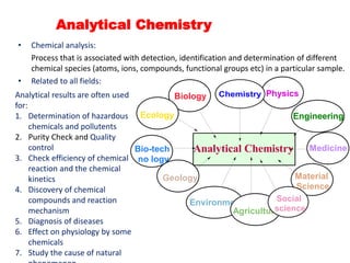
• Chemical analysis:
Process that is associated with detection, identification and determination of different
chemical species (atoms, ions, compounds, functional groups etc) in a particular sample.
• Related to all fields:
Analytical results are often used
for:
1. Determination of hazardous
chemicals and pollutents
2. Purity Check and Quality
control
3. Check efficiency of chemical
reaction and the chemical
kinetics
4. Discovery of chemical
compounds and reaction
mechanism
5. Diagnosis of diseases
6. Effect on physiology by some
chemicals
7. Study the cause of natural
2. • Types:
• Qualitative: Deals with identification of the substance (analyte).
• Quantitative: Concerned with the determination of amount /quantity of the
analyte. In the sample.
Analytical Chemistry
• Analytical Methodology: (Classical and Scientific)
o Complete analysis consists of series of steps
Problem identification,
Selection of a method,
Sample collection,
Processing the sample,
Making sample solution,
Preparation of standard,
Measure the property of interest,
Compare with standard,
Calculation and interpretation
Check validity and reliability
4. Errors and the treatment of
Analytical Data
CHAPTER
Results of coin flipping
5. Syllabus
Topics to be Covered
1. Errors in chemical analysis-absolute, relative errors.
2. Types of errors in experimental data :systematic errors (instrumental,
methodical and personal). Effect of systematic error-constant,
proportional error.
3. Sources of random error, distribution of experimental data.
4. Statistical treatment of random error. Central tendency and
variability, confidence limits, Student’s t, detection of gross error- Q-
test (rejection of data),
5 the least square method, correlation coefficients.
6. Propagation of determinate and indeterminate errors, Numerical
6. Errors in chemical analysis
Refers to the numerical difference between a
measured value and the true value
Often denotes the estimated uncertainties in a
measurement or experiment
What is a true value of any quantity???
is really something that we never know
TRUE VALUE: A value is accepted as being true when it is
believed that the uncertainty in the value is less than the
uncertainty in something else with which it is being
compared.
7. Sources of Errors :
a. The magnitude of error depends on: method
chosen and time spend for analysis.
b. Analysis process includes many steps and
methods.
c. Faulty calibration, standardization,……=>one
directional error
d. Random error
• The reliability of result signifies that the quality or
performance of the process is considerably good,
true and dependable to some ..…{a reliable
assistant, a … data, a… source}
8. Absolute Error
• Difference between
experimental value and
true value
• Shows whether the value
is high or low
• Sign is retained
• Less informative as it has
no relation with sample
size
Where,
Xi= observed value
Xt= true value
a i t
ia t
For individual data:
AbsoluteError (E ) X X
For average of data:
AbsoluteError (E ) X X
both positive and negative sign.
9. a
19.4 19.5 19.6 19.7 20.1 20.3
Here, 19.8 ppm
6
20.00 ppm
E 19.8-20.0 -0.2 ppm
t
x
x
Q. If standard Fe (II) solution of 20.0 ppm is analysed, the six replicate
measurements are shown in figure, calculate absolute error.
Negative sign indicates that measured
value is less than the true value.
ia t
We have;
AbsoluteError (E ) X X
10. Relative Error
• More useful
• Expressed as %, ppt, ppm relative to the
sample size
n
t
ti
r
x
xx
E 10
• It is independent upon the size of sample
• It is generally expressed in percentage or parts per thousand.
• Relative error also possesses the sign.
In general
n= 2,3,6……….
i t
r
t
i t
t
(X – X )
Relative Error (E ) 100; In %
X
(X – X )
1000; In PPT
X
11. Few Questions
1) Suppose that 0.5mg of precipitate is lost as a result of being
washed with 200ml of wash liquid. If the precipitate weighs
500mg , what will be the relative error due to solubility loss.
2) A method of analysis yields weights for gold that are low by
0.4mg. Calculate the percent relative error caused by this
uncertainty if the weight of gold in the sample is (i) 250 mg
(ii)700mg.
3) A loss of 0.4mg of Zinc occurs in the course of an analysis for
that element. Calculate the percent relative error due to this
loss if the weight of Zinc in the sample is 40 mg.
4) (i) A relative error of 0.5% is how many parts per thousand?
(ii) A relative error of 2.0 parts per 500 is what percent error?
13. – The correctness of an experimental result is called accuracy
– An accurate result is the one that agrees closely with the true
value of a measured quantity
– Accuracy is the closeness of a measured value to the true value
– expressed in terms of error (Less is the error greater is the
accuracy and vice versa).
– Accuracy can never be determined exactly, because the true
value of a quantity is almost unknown.
– Expressed by errors both absolute and relative
“Systematic errors affects the accuracy of results”
14. – Measures the reproducibility of the result i.e. closeness or
agreement of the results in the replicate measurement
(obtained in exactly the same way)
– Agreement among a group of experimental results.
– tells nothing about the relation with the true value (scatterness
from the average value). Can be determined just by measuring
replicate samples
– Precise value may be inaccurate
– Commonly stated in terms of expressed/measured in terms of
statistical parameters like; standard deviation, average
deviation or range
“Random Error affect measurement precision”
16. Fig: Pattern of Darts (missile) on the dart board
a) Low accuracy low precision
b) High accuracy low precision
c) Low accuracy high precision
d) High accuracy high precision
True value
Dart board
17. N
C OH
O
Nicotinic acid
{prevents pellagra)
CH2 S
NH2Cl
NH
Benzyl isothiourea hydrochloride
Determination of
Nitrogen in Benzyl
isothioureahydhrochlorid
e and Nicotonic acid by
Kjeldahl method.
Each dot represent error
for single determination
and vertical line
represent average
deviation.
In Kjeldahl method:
Sample containing Nitrogen → Hot and conc. H2SO4 (HgO, Se,Cu2+) → Ammonium sulphate
→ Ammonia
Analysis 3 & 4 give negative deviation (bias), because of incomplete decomposition by H2SO4;
(N is in pyridine ring).
This error can be minimized by
•addition of K2SO4 will increase the boiling temperature.
•O-N & N-N are pre treated to reducing condition.
18. ERROR IN EXPERIMENTAL DATA
Systematic
(Determinate)
Random
(Indeterminate)
Gross
• Affects accuracy.
• definite value ,
assignable cause,
and can be
measured.
• Biased: unidirectional
(same sign error)
• under the control
and can be
corrected
• affect sensitivity
• No definite cause
• Symmetric
distribution
• affects accuracy
• Mistake in
operation
• Few are out liers
•
19. Systematic Error
• Have definite value and an assignable cause, can be measured.
• Are of the same magnitude for replicate measurement made in
the same way
• Affect the accuracy of result
• Causes the mean of the data set to differ from the accepted
value
• Generally unidirectional w.r.t true value i.e. either too high or
too low located in same side(same sign error/ bias) under the
control of analytical chemist and can be corrected after careful
investigation.
• Reproducible and can be predicted and also can be avoidable
after careful investigation
20. Types of Systematic Errors
Instrumental
Error
Method Error
Personal Error
Due to improper calibration
of instrument.
Side reactions, heating to
high temperature.
They are detectable and
correctable
Calibration eliminates most of
this types of errors
• Caused from non ideal
chemical or physical
behavior of analytical
system
• Most serious of the
three types
• Difficult to detect
• We can use the
following steps to help:
1-Analyzing Standard
• Results from
carelessness,
inattention, or
personal limitation of
the experiment
• example: estimation
errors, observation
errors, etc Misreading of an instrument or scale
Insensitivityto colour changes
Improper calibration
Poor technique/samplepreparation
Improper calculationof results
Preconceivedidea of ‘true’ value – personal bias
These are blunders that can be minimised or eliminatedwith
proper training and experience.
21. Detection and removal of instrumental error:
These types of error are detectable and correctable. Simply frequent calibration can
remove large magnitude of these errors.
Calibration eliminates most of this types of errors
They are detectable and correctable.
• It one of the potential source of error, is originated from the non ideal
instrumental behavior i.e. failure of measuring devices to be in accordance
with required standard leads to instrumental error.
• Due to faulty construction, no proper calibration, attacking by reagent etc.
causes instrumental error.
• Using glassware outside of calibrating temperature (measuring devices like
pipette, burette, VF are affected).
• By contamination of inner surface due to reagents will give volume error
from original calibration.
• Attack by reagents; corrosion and distortion: give volume error and weighing
error.
• Decrease of voltage or increase of resistance due to temperature change
affects the accuracy and precision.
• If electrical devices are used with insufficient voltage, long time without
calibration, or used outside the working range; pH meter suffers large error
at higher acidic or basic range.
22. Detection and removal of Method error:
Method errors are difficult to detect among three. Validation of the method can be done by using
standards (from NIST). It sells variety of reference materials.
1-Analyzing Standard Samples
2-Using an Independent Analytical Method
3-Performing Blank Determinations
4-Varying the Sample Size.
• The method imposed for chemical analysis. Non ideal chemical and
physical behavior of the reagents and reactions upon which the method is
based introduces the systematic method error. Some examples are:
• Slowness of reaction or incompleteness of some reagents in a reaction.
• Incomplete drying before weighing.
• Instability of some species.
• Possibility of side and chain reactions.
• Non specificity of most reagents.
• Excess titrant is required if more amount of indicator is used.
• Heating sample to high temperature and weighing hygroscopic substances.
• Lack of reproducibility in solvent extraction (due to appreciable solubility of
ppt).
e.g. in N – estimation of Nicotinic acid it is decomposed by conc. H2SO4
into(NH4)2SO4 which is then determined. The decomposition is incomplete
unless special precautions are not applied. This always gives negative error.
23. example: estimation errors, observation errors, etc
Misreading of an instrument or scale
Insensitivity to colour changes
Improper calibration
Poor technique/sample preparation
Improper calculation of results
Preconceived idea of ‘true’ value – personal bias
These are blunders that can be minimised or eliminated with proper training and
experience.
• Lack of care and constitutional inability of an individual to make certain
observation individually give rise of meaningless error which is called person
systematic error. (because of carelessness, inattention, habits and knowledge
of experimenter)
• Estimation of pointer position between two graduations
• Locating the end point by color change of indicator in titrimetric analysis (less
sensitive experimenter will give more result)
• The next source of personal error is prejudice or bias
• Results from carelessness, inattention, or personal limitation of the experiment
• Detection and removal of personal error:
Every chemist even much honest have a natural tendency to estimate scale
reading in the direction that improves the precision of a set of results, is one of the
serious cause of personal error.
24. –Systematic errors may either be constant or
proportional
• The magnitude of a constant error does not
depend on the size of the quantity measured
• Proportional errors increase or decrease in
proportion to the size of the sample taken for
analysis
25. • The magnitude of determinate error is nearly constant in a series of analysis
and is independent on magnitude of measured quantity.
• becomes less significant as the magnitude increases and is more serious for
small sample.
• One way of reducing the effect of constant error is to increase the sample
size until the error is tolerable.
• With constant errors, the absolute error is constant with sample size , but the
relative error varies when the sample size is changed.
• Effect of constant error becomes more serious as the sample size decreases.
• 0.1 ml end point error in titration (use of excess reagent to predict the end
point). It causes 1% error for 10 ml sample but only 0.2% for 50 ml sample.
• Also if 0.5mg of precipitate is lost in washing by certain volume of solvent, if
initial precipitate weights 500mg gives relative error of -0.1% but if initial
precipitate weights 50mg it gives -1.0% error.
• Weighing error and rounding the significance figures.
26. Example of Constant Error
(i) If a constant end point error of 0.1ml is made in a series of
titrations, this represents a relative error of 1% for sample
requiring 10ml of titrant, but only 0.2% if 50 ml of titrant is used.
(ii)Effect of solubility loss in gravimetric analysis
• Suppose that 0.50 mg of precipitate is lost as a result of being
washed with 200 mL of wash liquid. If the precipitate weighs
500 mg, the relative error due to solubility loss is
–(0.50/500) x 100% = -0.1%. Loss of the same quantity from 50
mg of precipitate results in a relative error of –1.0 %.
(iii) addition of excess reagent to bring about color change during a
titration. This small volume remains the same regardless of the
total volume of reagent required for the titration.
27. – The absolute value of this type of error varies with the
sample size in such a way that the relative error remains
constant.
– It decreases or increases in proportion to the size of the
sample.
– A common source of proportional errors is the presence
of interfering contaminants in the sample.
28. Example of proportional Error
(i) example in determining of Cu(II) by KI; presence of Fe(II) also
liberates I2 from KI which give positive error. If the sample size is
doubled, for example, the amount of iodine liberated by both the
copper and the iron contaminant is also doubled. Thus, the
magnitude of the reported percentage copper is independent of
sample size.
(ii) In the iodometric determination of an oxidant like chlorate,
another oxidizing agent such as bromate would cause high results
if its presence were unsuspected and not corrected for.
Taking larger samples would increase the absolute error, but the
relative error would remain constant provided the sample was
homogenous
29. Random Error
• Random error exists in every measurement and are often major source of
uncertainty.
• These errors which have no particular assignable cause.
• Can never be totally eliminated or corrected
• Caused by many uncontrollable variables that are inevitable part of every
analysis made by human beings; are random error.
• These variables are impossible to identified, even if we identify some they
cannot be measured, because most of them are so small
• Random in nature and lead to both high and low results with equal
probability. the accumulated effect of small random error is high and will
fluctuate randomly around the mean.
• In absence of systematic error random error only affects the precision.
• Random error arises obeying the probability theory of statistics
• Increasing the number of sample will minimize the magnitude of random
error.
Eg, Noise and drift in an electric circuit
Vibration in building caused traffic etc……..
30. How small undetectable uncertainties produce a detectable random error can be
explained from the example:
Imagine a situation in which four small random errors combine to give a overall error. Let
each factors can fluctuate the final result by ± 1 with equal probability of occurrence. The
following combinations (addition/subtraction) are possible.
Combination of
uncertainties
Magnitude of
Random error
Number of
Combinations
(Frequency)
Relative
frequencies
+ U1 + U2 + U3 + U4 +4U 1 1/16 = 0.0625
- U1 + U2 + U3 + U4
+2U
4 4/16 = 0.250
+ U1 - U2 + U3 + U4
+ U1 + U2 - U3 + U4
+ U1 + U2 + U3 - U4
- U1 - U2 + U3 + U4
0
6 6/16 = 0.375
-U 1+U 2-U 3+U 4
-U 1+U 2+U 3-U 4
+U 1-U 2-U 3+U 4
+U 1-U 2+U 3-U 4
+U 1+U 2-U 3-U 4
+U 1-U 2-U 3-U 4
- 2U
4 4/16 = 0.250
-U 1+U 2-U 3-U 4
-U 1-U 2+U 3-U 4
-U 1-U 2-U 3+U 4
-U 1-U 2-U 3-U 4 - 4U 1 1/16 = 0.0625
If a curve of relative frequency versus deviation from mean is plotted, it will give a bell
shaped curve. As the number of individual error is very large, the curve takes the shape
as in figure, this curve is called normal error curve or Gaussian curve (properties are
discussed later).
31. • Calibration of a pipette:
10 mL of water is pipetted → poured in stoppered flask of known
weight → weight change is calculated for all steps → Volume is
calculated by dividing with density, at that temperature → Data is
tabulated (converting into discrete frequency or continuous frequency)
→ This can also be plotted as bar diagram or histogram or frequency
polygon → in absence of systematic error, with increasing number of
data the frequency polygon curve is bell shaped, symmetric in both
sides → This curve is called as normal error curve.
• In this determination there are numerous possible sources of random error. →
visual error (level of water, mercury level in thermometer…) → temperature
fluctuation (affects; volume of pipette, viscosity of liquid, performance of
balance…) → variation in drainage time and the angle of pipette at drainage →
vibrations and drafts (affects the balance reading)
• Any other examples can be considered.
→ Production run of multivitamin tablets
→ Determination of Ca2+ in community water supply
→ Determination of glucose in the blood of diabetic patient
→ Measurement of absorbance of 50 replicate 10ppm Fe(II) sample
complexing with thiocyanate ion.
32. Measurement of central tendency: A single value or data that can represent the
mass of data is called Measure of central tendency. Central tendency is that single
quantity which can represent the whole sample.
intervalclassofwidth=
1
mean,assumed=and)(deviation
1
Others,
on)distributifrequency(for
mean;Populationmean;Sample
1
1
1
1
11
hdf
N
h
Ax
df
N
A
AAxdd
N
Ax
N
xf
N
x
N
x
x
N
i
ii
N
i
ii
i
N
i
i
N
i
ii
N
i
i
N
i
i
N
1.Mean: Average of all the values:-
- It is strictly defined, clearly defined and is most commonly used than other measures of central tendency.
- It is not much affected by fluctuating of sample, but means of N results are only
times reliable than individual result. Greater the number of sample more is the reliability.
- The extreme values highly affect the mean.
33. 2
1N
2
1N
Cf
2
N
2
N
Cf
class.precedingofCf=class,middletheoffrequency=
class,middletheofwidth=class,theoflimitlower=)
2
N
(
cf
hlc
f
h
lMd
1.Median: - The individual data (value) that divides the number of
observations into two equal parts; if are arranged in a sequence is called
median. For odd number of data middle value represents the median and for
even number of data average of two middle values represents the median.
For the case of discrete frequency distribution, we find the value of
, the cumulative frequency (Cf) is calculated, the individual item with
represent the median.
For continuous frequency distribution; find , see the class with
; it represent the median class, and median is calculated by the formula,
34. 1.Mode: The value of observation that repeats for the maximum
number of times is the mode. For the continuous frequency distribution,
mode.calculatetodifficultisitif23also,
class.lsucceedingtheoffrequency=
clasprecedingltheoffrequency=class,modaltheoffrequency=
)()(
)(
0
2
01
2101
01
0
xMM
f
ff
ffff
ffh
lM
d
34
36. – Population Parameters
• µ =mean of infinite population
• s = standard deviation of population
• X- µ that represents the extend to which an individual value X
deviates from the mean
– Sample Parameters
• = sample mean
• S= sample standard deviation
x
36
39. The data can be tabulated as, Individual series, Discrete frequency
distribution, Continuous frequency distribution, or in the form of Diagrams;
Bar diagram, Histogram, Frequency polygon …
Histogram Frequency polygon
Roll
No Marks
1
2
.
Marks No of
Students
0-10 2
10-20 1
…..
Individual series
Continuous frequency
39
40. Arrange the data in sequence,
lowest to highest or …
Condense the data into
class/cells by grouping, decide
the number of cells (10-20) and
choose the boundaries.
Confusion can be eliminated by
choosing boundaries halfway
between two possible values.
Pictorial representation of
frequency distribution in terms of
histogram & frequency polygon.
In frequency polygon the middle
value of a cell connected
together.
40
42. Example : Study of Coin Flipping
Measure = How many heads will occur in ten (10) flips?
42
43. – The limiting case approached by the frequency polygon as more and more
replicate measurements are performed is the normal error curve or Gaussian
distribution curve.
– If we plot the curve as the function of relative frequency versus deviation
from the mean and assume that the probability of falling the data under the
curve is 1. The curve is called normal error curve,
. Here the area of the curve is proportional to number of
data between that ranges.
– The area under the curve between any two value of x-µ gives the fraction
of total population having magnitudes between these two values.
• µ±σ includes 68.26% of result
• µ±2σ includes 95.46% of result
• µ±3σ includes 99.74% of result
99.74% of
result
95.46% of
result
68.26% of
result
x
z
s
Where,
43
45. t
N
i
N
j
ji
pooled
nNN
xxxx
s
......
.........)()(
21
1 1
2
2
2
1
1 2
No of degree of freedom is equal to total no of sample (N1 + N2 + ….) minus no of subsets (nt)
• Here we will discuss, how to obtain reliable estimate of σ from small samples
of data.
• Performing preliminary experiments: If we have more time and adequate
sample, reliable SD for the method can be obtained in the preliminary step by
increasing N; if N is about 20; s and σ can be assumed identical.
• Pooling data: If we have several subsets of data, we can get better estimate of
population SD by pooling (combining) the data; assuming that, data are
replicate and each sub set has the common σ.
• Spooled is the weighted average of the individual estimates.
45
46. Specimen
number
No. of sample
measured
Hg content, ppm Mean ppm
of Hg
Sum of sq. of deviation
from mean
1 3 1.80, 1.58, 1.64, 1.673 0.0259
2 4 0.96, 0.98, 1.02, 1.10, 1.015 0.0115
3 2 3.13, 3.35 3.240 0.0242
4 6 2.06, 1.93, 2.12, 2.16, 1.89, 1.95 2.018 0.0611
5 4 0.57, 0.58, 0.64, 0.49 0.570 0.0114
6 5 2.35, 2.44, 2.70, 2.48, 2.44 2.482 0.0685
7 4 1.11, 1.15, 1.12, 1.04 1.130 0.0170
Σ = 28 Σ = 0.2196
Q. The mercury in the sample of seven fish taken from Mississipi River was determined with
a method based on the absorption of radiation by gaseous elemental mercury.
(a) Calculate the pooled estimate of the standard deviation for the method, based on the
first three columns of data in the table it follows:
(b) (b) Calculate the 50% and the 95% confidence limits for the mean value (1.67ppm) for
the sample 1, consider s ≈ σ = 0.10
(c) How many replicate measurements of specimen 1 would be needed to decrease the
95% confidence interval to ± 0.07ppm Hg?
t
N
i
N
j
ji
pooled
nNN
xxxx
s
......
.........)()(
21
1 1
2
2
2
1
1 2
46
47. • For most analytical task, we do not know the, however, we can use
the experimental mean and standard deviation to estimate the
range of true value.
• Since μ (true value) cannot be determined;
• In absence of systematic error; we can define the numerical
interval around mean of replicate results within which the
population mean is expected to lie with the given degree of
probability, is called confidence interval and the boundaries are
called confidence limits.
• For example conc. of population at 90% cf is 7.25 ± 0.15; which is,
7.10% -7.40%. It is calculated from sample standard deviation.
• Confidence interval- calculated range of estimated true value
• Confidence limit- limit of this range
• Confidence level- the likely hood that the true value falls in this range
47
48. s
x
z
meantheoferrorstandardwithandxbyreplacedisxhere, s
s
N
z
xofCI
,
Used to compare of experimental mean with known
value.
• For large number of sample data. N > 20
• From equation
• The confidence interval of true mean based on single
value (x) can be written as,
CI for μ = x ± zσ.
• If we use experimental mean
• of N data is the better estimator of μ, than single
measurement;
• CI can be narrowed by taking more measurement (taking
4 measurements will half the CI of μ)
• This equation is applied only if bias is zero (s is good
approximation of σ)
confide
nce
level,
%
z confide
nce
level,
%
z
50 0.67 96 2
68 1 99 2.58
80 1.29 99.7 3
90 1.64 99.9 3.29
95 1.96
48
49. – W. S Gosset (1908) studied the problem of making predictions based
upon a finite sample drawn from unknown population.
– In practical works we know and s rather than µ & σ (where, and s
are estimates of µ & σ )
– These estimates are subjected to uncertainty and predictions can be
made about the falling of an odd observation outside the limit.
– Conficence limit for small no of data set is explained by a new
statistical parameter “t”, analogous to z.
– s calculated from small set of data may be quite uncertain and it
broadens the confidence interval.
– The quantity t which is calculated to compensate uncertainty using “s”
instead of “σ”
x x
49
50. s
x
t
N
s
x
t
meantheoferrorstandardwithandxbyreplacedisxhere, s
N
ts
xofCI
t , for a mean of N measurement,
• This parameter t is called student’s t, which explains about the uncertainty on s
as the estimate of σ.
• Magnitude of t depends on degree of freedom in calculating s (DF for small
sample is N-1).
• The confidence interval for the mean .. of N replicate measurement can be
calculated by t-equation,
t , for a single measurement, is defined as:
where = sample mean
µ = population mean or true mean
s= sample standard deviation
n=no. of observation
t depends on degree of freedom in the calculation of ‘s’
Degree of Freedom: refers to the number of
values in a sample that can be choosen freely,
( the no. of observations remains unspecified)
Degree of freedom= sample size – number of
population parameter that are estimated from
sample observations.
50
51. • x- mean value; s- standard
deviation
• N- number of measurements
• t – located using table
• Determine the value of v-
degrees of freedom (N-1) than
identify the t- value with the
respective % confidence level.
51
52.
• Null hypothesis (H0) :- μ = μ0
• Alternative hypothesis (Ha) :- μ≠μ0, (It may be into two kinds, μ< μ0,or μ> μ0 one
tailed.)
• We apply z test for the large sample where s and σ are good approximate.
• We apply t test for the small sample where s and σ are not good approximate.
• Null hypothesis is accepted if test statistics lie within the accepted region and is
rejected if lies in the rejection region. We compare these values with the
tabulated values at given degree of freedom.
• If t or z calculated > t or z tabulated we reject the null hypothesis, ie………
• If t or z calculated < t or z tabulated we accept the null hypothesis i.e.
Testing for Significance, by t statistics
52
53. Testing for Significance
t-test can be used for the comparison of two means.
• Sample is analyzed by two different methods, each repeated several times, and the
mean value obtained are different.– Is the difference between two values significant?
• t-test enables us to decide whether the difference in mean is simply due to random
error or there exists certain systematic error in any one of them.
21 xx
21 xx
1 2
1 2
1 2
x x N N
t
s N N
ii. Comparison of two mean:
We predict, Null hypothesis: mean of analyst 1 = mean of analyst 2; ( ), It is.
Alternative hypothesis is ( ) (two tailed),
if s1and s2 are their standard
deviations, t test for the
difference between mean is
computed by using formula,
Here number of degree
of freedom (df) = N1 + N2 - 2
we accept the null hypothesis
i.e. there is no significance difference between two mean.
If tcalculated < ttabulated;
t- is calculated using formula
53
54. Confidence interval of the Mean
– Confidence interval for the mean is the range of values
within which the population mean µ is expected to lie
with a certain probability.
– Confidence limit is the probability that the true mean lies
within the certain interval.
– It is given as
– CL is used to estimate the probability that the population
mean lies with in a certain region centered at x or sample
mean.( certain range either side of x bar)
limit of
ts
Confidence x
N
54
55. Gross Error
• A third type of error is gross error; it differs from determinate and
indeterminate errors,
• Gross errors occur occasionally and are too large (higher or lower)
• Only few of the results will scatter outside from the rest.
• Te result that differs markedly from all other replicate data are called
outliers.
• There is no evidence of gross errors. But are produced by human
error. For eg, If a part of ppt is lost before weighing or if a weighed
bottle is touched by fingers.
• The outliers can introduce error in the analysis, so criteria should be
made weather to retain or reject the data (that is remaining free from
bias).
• A single result appears to be out side the range of what random errors
in procedure gives
• Generally arise due to human error
55
56. • Criteria must be developed to decide on the rejection or retaining of
outlying data
• Proper statistical treatment needed before rejection
• The consequence of making error in statistical tests are often compared
with the consequences of error made in judicial procedure.
• In this test the absolute value of the difference between questionable
and the nearest value is compared with spread; which is called Q.
• This Q value is compared with tabulated value; if Q > Qtab or Qcrit, the data
is rejected; otherwise retained.
Steps:
1. Calculate the range of the result (W)
2. Calculate difference between suspected result and the nearest
neighbor.
3. Divide II by I, to get rejection quotient (Q)
4. Find the tabulated value and compare.
Gross Error
• Qcal > Qtab, result can be discarded with 90% confidence
• Qcal < Qtab, Accept result
56
57. The minimum difference between suspected data and other
data has to be assigned before the result is to be discarded
which may introduce other types of error.
– If the minimum difference is made too small, the valid data may
be rejected too frequently, such error are TYPE I.
• Occurs when null hypothesis is rejected although it is
actually true (false negative)
– If the minimum difference is made too high, there is too
frequent retention of highly erroneous values, such error are
TYPE II.
• Occurs when null hypothesis is accepted although it is
actually false (false positive)
Gross Error
57
58. Propagation of Error
• The method of transferring errors from individual
observation into final result through series of calculations is
called propagation of errors.
• Attention focused on accuracy and precision of final
computed result, but it is instructive to see how errors in the
individual measurements are propagated into the result.
1. Determinate error (i)Addition and subtraction
(ii)Multiplication and Division
2. Indeterminate error (i)Addition and subtraction
(ii)Multiplication and Division
58
59. Let us consider the final result R and the A, B, C are the preliminary
measurements. If error associated with are represented by ρ, α, β and δ
respectively.
•In the case of addition and
subtraction, we have
).........(..........gives(ii)(i),solving
)(..........).........()(
)()()(errorsrespectivethegIntroducin
).........(..........
iii
iiCBA
CBAR
iCBAR
That is if addition and subtraction were involved, determinate errors are
transmitted directly into the result.
-ve sign for γ introduces the maximum positive error and -ve sign for α and β
introduces the maximum negative error in the final result.
Suppose R = A + B - C
Where, R=computed result
A,B and C are measured quantity
59
60. •In the case of
multiplication and
division,
CBAR
CCC
AB
C
CC
ABACBC
R
iv
vi
CC
ABACBC
CC
ABABCACBCABC
C
AB
C
ABAB
viv
v
C
ABAB
R
C
ABAB
C
BA
R
ivCABR
so,tocomparedassmallveryisSince
)(
)(it withCombining
).......(..........
)(
)(
gives)(&)(Solving
).......(..........
)(
)(
so;negligibleare&
.
)(
)(
)(
)()(
errorsrespectivethegIntroducin
).........(..........
i.e. if multiplication and division are involved , relative determinate error are
transmitted directly into the result.
[For the case to obtain maximum relative error, the expression C- γ should be
used in place of C + γ]
60
62. •For the case of multiplication and division,
).........(..........
ssss
byDividing
sss
ssss
:casepreviousin theAs,deviationsstandardtheirare,,,,if
).........(..........
222
2
2
2
2
2
2
2
2
2
2
2
,
2
2
,
2
2
,
2
iv
CBAR
C
ABR
C
AB
C
A
C
B
C
R
B
R
A
R
ssss
iii
C
ABR
CBAR
CBA
C
BA
B
CA
A
CB
R
CBAR
Thus for the product and quotients, the relative standard deviation of the result is equal to
the sum of squares of the relative standard deviations of the number making up the product
or quotient.
The squares of the
relative variances are
transmitted
62
63. Y
X
Concentration
InstrumentalResponse
• Most of chemical analysis requires a plot of
linear curve (i.e. the detector response or the
final result is linearly related with the
concentration of the analyte)
• By using different standard solutions we can
plot the curve, called calibration curve. But due
to accumulation of errors all readings may not
be located in the line. In such a situation we
have to draw the line of best fit, which is
determined by the method of least square.
Only then the concentration of unknown can
be determined accurately.
• The uncertainties of the analysis can also be
determined from this regression line.
• In the least square method the slope and
intercept of the line is determined
mathematically. If the equation for the best fit
be, y = mx + b……….. (i); where m= slope
and b = intercept
• The least square method assumes that;
– The sum of squares of residuals from all the
points is minimum. [The vertical deviation from
each point to the line is called residual]..
Not only can the best line be
determined but also the
uncertainties in the use of the
calibration graph for the
analysis of an unknown can be
specified. 63
y mx b
64. P(xi,yi)
y = mx + b
Residual = PQ= yi-(mxi+b)Y
Fig: Calibration curve for isooctane (peak area vs % mole)
0.5 1.0 1.5 2.0 2.5 3.0
X
• The least square method assumes
that;
– The sum of squares of residuals from
all the points is minimum. [The vertical
deviation from each point to the line is
called residual].
2
[ ( )]resid i i
i
SS y mx b
0&0&0minima,ofprincipletheFrom
b.andmestimatetohaveWe(ii).............0&0
2
2
2
2
b
SS
m
SS
b
SS
m
SS
b
SS
m
SS
residresidresidresid
residresid
(iv).............0][..
0-1)]([2..
0
)]([
,
(iii).............0][..
0-)]([2..
0
)]([
..
2
2
2
bmxyei
bmxyei
b
bmxy
Also
bxmxyxei
xbmxyei
m
bmxy
ei
ii
ii
ii
iiii
iii
ii
•The sum of square of residual is given by, SSresid
•To minimize SSresid ; the first derivative is set to zero w.r.t. the
variables m and b.
•Solving the equations gives,
Equations (iii) and (iv) are normal equations to fix the line. i.e. solving the values of m
and b from the above equations we can get the line of best fit.
65. 2
2 2
2
2 2
i i
( )
( )
( )
( )
( )( )
Where x and y are individual parts of x and y
N is number of pairs
& are average values of
i
xx i i
i
yy i i
i i
xy i i i i
x
S x x x
N
y
S y y y
N
x y
S x x y y x y
N
x y
x and y
)(11
curvencalibratiosameusingobtainedresultsreplicateofSD(g)
)(
interceptofSD(f)
slopeofSD(e)
freedomofdegree2)-(NCLslopeforC.L.90%(d)
2
line)regressionthefromdeviationtypicalaofmeasurerough(ay.ofSDcalledalsois
estimatetheoferrorstandardregressionaboutSD(c)
bIntercept,(b)
C
xx
xy
or,mlineofSlope(a)
2
2
22
2
2
0.90
2
xx
cr
c
ii
i
b
xx
r
m
m
xxyy
r
xx
xy
Sm
yy
NMm
s
s
xxN
x
s
S
s
s
tsm
N
SmS
s
xmy
N
S
S
If we
represent,
65
66. • If a linear relationship between x and y does
exist, this puts the line through the best
estimates of the true mean values.
If we
represent,
66
67. • The standard deviation of the y-values, sy is
given by (where deg. of freedom
=n-2)
• The standard deviation of slope, sm is given by
• The 90% confidence limit of the slope is
67