![Laminar Flow of A Bingham Fluid Over A Rotating Disk
www.ijmsi.org 2 | P a g e
The value of vanishes near the surface of the disk, since there is no penetration. However, the value of
as is not specified; it adjusts to a negative value, which provides sufficient fluid necessary to maintain the
pumping effect. As shown below, it becomes part of the solution to the problem. In contrast to the axial velocity,
both the radial and tangential velocities go to zero at large axial distances from the disk.
Equations of Motions:
Applying the assumptions the transport equations for conservation of mass and momentum, in
cylindrical co-ordinates, can be written as follows (Bird et al., 2002): [160]
Continuity equation:
(3)
Momentum equations:
in the r-direction:
(4)
in the -direction:
(5)
in the -direction:
(6)
Boundary Layer Approximations:
Since the motion of the fluid is caused by the rotation of the disk, at sufficiently high Reynolds number
the viscous effects will be confined within a thin layer near the disk. Therefore, further simplification can be
obtained by considering the usual boundary-layer approximations (Owen and Rogers. 1989) [161] :
• The component of velocity is very much smaller in magnitude than either of the other two components;
• The rate of change of any variable in the direction normal to the disk is much greater than its rate of
change in the radial or tangential directions
and
• The only significant fluid stress components are and
• The pressure depends only on the axial distance from the axis of rotation.
Therefore, equation (3) is unchanged; it is repeated as equation (7). Equations (4) to (6) reduce to
equations (8) to (10).
(7)
(8)
(9)
(10)
Similarity Transformations:
The classical approach for finding exact solutions of linear and non-linear partial differential equations is
the similarity transformation. They are the transformations by which a system of partial differential equations
with n-independent variables can be converted to a system with n-1 independent variables. The axisymmetric
momentum equations associated with rotating disk flow have mainly been solved using a similarity
transformation, which allows the governing partial differential equation set to be transformed into a set of
ordinary differential equations. In the similarity solution, analytical relationships will be used and dimensionless
parameters will be substituted so that the number of variables to be solved is reduced.
The solution is based on the appropriate non-dimensional transformation variable given by von Karman
(Cochran, 1934) [162] i.e.,
(11)](data:image/gif;base64,R0lGODlhAQABAIAAAAAAAP///yH5BAEAAAAALAAAAAABAAEAAAIBRAA7)
Recommended
Recommended
More Related Content
What's hot
What's hot (20)
Viewers also liked
Viewers also liked (20)
Similar to A0230107
Similar to A0230107 (20)
Recently uploaded
Recently uploaded (20)
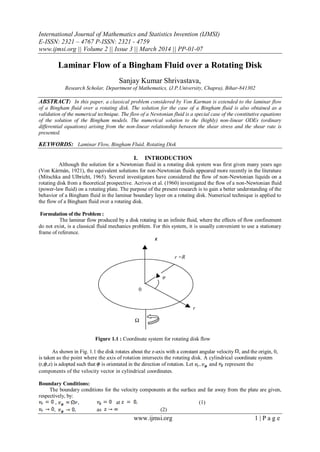
A0230107
- 1. International Journal of Mathematics and Statistics Invention (IJMSI) E-ISSN: 2321 – 4767 P-ISSN: 2321 - 4759 www.ijmsi.org || Volume 2 || Issue 3 || March 2014 || PP-01-07 www.ijmsi.org 1 | P a g e Laminar Flow of a Bingham Fluid over a Rotating Disk Sanjay Kumar Shrivastava, Research Scholar, Department of Mathematics, (J.P.University, Chapra), Bihar-841302 ABSTRACT: In this paper, a classical problem considered by Von Karman is extended to the laminar flow of a Bingham fluid over a rotating disk. The solution for the case of a Bingham fluid is also obtained as a validation of the numerical technique. The flow of a Newtonian fluid is a special case of the constitutive equations of the solution of the Bingham models. The numerical solution to the (highly) non-linear ODEs (ordinary differential equations) arising from the non-linear relationship between the shear stress and the shear rate is presented. KEYWORDS: Laminar Flow, Bingham Fluid, Rotating Disk I. INTRODUCTION Although the solution for a Newtonian fluid in a rotating disk system was first given many years ago (Von Kármán, 1921), the equivalent solutions for non-Newtonian fluids appeared more recently in the literature (Mitschka and Ulbricht, 1965). Several investigators have considered the flow of non-Newtonian liquids on a rotating disk from a theoretical prospective. Acrivos et al. (1960) investigated the flow of a non-Newtonian fluid (power-law fluid) on a rotating plate. The purpose of the present research is to gain a better understanding of the behavior of a Bingham fluid in the laminar boundary layer on a rotating disk. Numerical technique is applied to the flow of a Bingham fluid over a rotating disk. Formulation of the Problem : The laminar flow produced by a disk rotating in an infinite fluid, where the effects of flow confinement do not exist, is a classical fluid mechanics problem. For this system, it is usually convenient to use a stationary frame of reference. z r =R φ 0 r Ω Figure 1.1 : Coordinate system for rotating disk flow As shown in Fig. 1.1 the disk rotates about the z-axis with a constant angular velocity , and the origin, 0, is taken as the point where the axis of rotation intersects the rotating disk. A cylindrical coordinate system (r, ,z) is adopted such that is orientated in the direction of rotation. Let and represent the components of the velocity vector in cylindrical coordinates. Boundary Conditions: The boundary conditions for the velocity components at the surface and far away from the plate are given, respectively, by: , , at (1) , , as (2)
- 2. Laminar Flow of A Bingham Fluid Over A Rotating Disk www.ijmsi.org 2 | P a g e The value of vanishes near the surface of the disk, since there is no penetration. However, the value of as is not specified; it adjusts to a negative value, which provides sufficient fluid necessary to maintain the pumping effect. As shown below, it becomes part of the solution to the problem. In contrast to the axial velocity, both the radial and tangential velocities go to zero at large axial distances from the disk. Equations of Motions: Applying the assumptions the transport equations for conservation of mass and momentum, in cylindrical co-ordinates, can be written as follows (Bird et al., 2002): [160] Continuity equation: (3) Momentum equations: in the r-direction: (4) in the -direction: (5) in the -direction: (6) Boundary Layer Approximations: Since the motion of the fluid is caused by the rotation of the disk, at sufficiently high Reynolds number the viscous effects will be confined within a thin layer near the disk. Therefore, further simplification can be obtained by considering the usual boundary-layer approximations (Owen and Rogers. 1989) [161] : • The component of velocity is very much smaller in magnitude than either of the other two components; • The rate of change of any variable in the direction normal to the disk is much greater than its rate of change in the radial or tangential directions and • The only significant fluid stress components are and • The pressure depends only on the axial distance from the axis of rotation. Therefore, equation (3) is unchanged; it is repeated as equation (7). Equations (4) to (6) reduce to equations (8) to (10). (7) (8) (9) (10) Similarity Transformations: The classical approach for finding exact solutions of linear and non-linear partial differential equations is the similarity transformation. They are the transformations by which a system of partial differential equations with n-independent variables can be converted to a system with n-1 independent variables. The axisymmetric momentum equations associated with rotating disk flow have mainly been solved using a similarity transformation, which allows the governing partial differential equation set to be transformed into a set of ordinary differential equations. In the similarity solution, analytical relationships will be used and dimensionless parameters will be substituted so that the number of variables to be solved is reduced. The solution is based on the appropriate non-dimensional transformation variable given by von Karman (Cochran, 1934) [162] i.e., (11)
- 3. Laminar Flow of A Bingham Fluid Over A Rotating Disk www.ijmsi.org 3 | P a g e along with the associated set of dimensionless velocity components and pressure, i.e., (12a) (12b) (12c) (12d) This similarity transformation implies that all three dimensionless velocity components depend only on the distance from the disk . The boundary conditions are transformed into the coordinate as follows: , at , as Note that the formulation above becomes problematic at the axis of the disk, where among other things the boundary layer assumptions break down. Bingham Model : Consider the flow of a Bingham fluid over a rotating disk. A Bingham fluid does not deform until the stress level reaches the yield stress, after which the „„excess stress‟‟ above the yield stress drives the deformation. This results in a two-layered flow consisting of a „plug layer‟ and a „shear layer‟. Figure 1.1 shows a sketch of a Bingham fluid flowing over a rotating disk, using a cylindrical coordinate system (r, , z). In a number of cases, the Bingham constitutive equation adequately represents the stress-deformation behaviour of materials with a yield stress. Ω r Disk Shear flow region τ > τy Plug flow region τ < τy z Figure 1.2: Simplified schematic of the flow geometry of a Bingham fluid on a rotating disk This model relates the rate-of-deformation tensor, defined below in terms of the velocity field vector , ------------------------------------------------------ to the deviatoric stress tensor, , using the following relations :
- 4. Laminar Flow of A Bingham Fluid Over A Rotating Disk www.ijmsi.org 4 | P a g e (16) When the magnitude of the shear stress is greater than the yield stress , the material flows with an apparent viscosity given by: where is the viscosity of the deformed material, referred to as the plastic viscosity. The magnitudes of the shear stress and deformation rate are defined, respectively, -------------------------------------------------------------- - ------------------------------------------------------------- -- As using the summation convention for repeated indices. With the approximations noted in the preceding section, and assuming rotational symmetry, one then obtains using the conventional index notation to describe the individual components. It should be noted that it is not possible to explicitly express the deviatoric stress in terms of the rate-of- deformation for a region where the stress is below the yield value, . The areas where have a zero rate- of-deformation, hence they translate like a rigid solid. Thus, this numerical method will neglect any unsheared region which might exist outside the boundary layer region, and instead focus on the sheared region which flows with apparent viscosity, It follows that the apparent viscosity for a Bingham plastic fluid takes the following form For cylindrical coordinates, the two pertinent stress components in the plastic region assume the following forms: For following boundary layer theory, the tangential component, and the radial component, , of the stress tensor become ------------------------------------------------------------- -
- 5. Laminar Flow of A Bingham Fluid Over A Rotating Disk www.ijmsi.org 5 | P a g e Substitution of equation (21) into (24) and (25), gives ------------------- These are the components of stress required to close the momentum equations given by Eqs. (8) and (9). A useful parameter is the “Bingham Number”, which is the ratio of the yield stress, , to viscous stress. It is used to assess the viscoplastic character of the flow and is defined as: which is expressed by the following relation [152]: where is the kinematic plastic viscosity of the fluid, is a characteristic length scale, and indicates that this a local Bingham number. It is possible to reduce the continuity and momentum equations to a set of ordinary differential equations by substitution of equations (12 a, b, c, d) for velocity, equations (26) and (27) for the shear stress components, and equation (29) for the ratio , into equations (7) to (10). This was accomplished with the aid of Maple software, and the resultant equations are presented below. Continuity Equation: Momentum Equations: r-wise -wise -wise ------------------------------------------- where a prime denotes differentiation with respect to . Since the last equation, (33), is the only one involving P , it may be integrated directly to give ----------------------- where is the value of at the disk. Hence no numerical integration for is necessary once F and H are determined. For solution purposes, it is advantageous to eliminate the second derivatives on the right hand side of equations (31) and (32) so as to obtain a single second order variable for each equation. Algebraic calculations
- 6. Laminar Flow of A Bingham Fluid Over A Rotating Disk www.ijmsi.org 6 | P a g e yield: ----------- ------ The resultant equations can be considered as a generalized case including both Bingham and Newtonian fluids, since setting will simplify these equations to represent a Newtonian fluid, i.e., The constitutive equation of the Bingham fluid has generated additional nonlinear terms in the momentum equations in comparison to the equations for a Newtonian fluid. Equations (35) and (36) are second order in both F and G, and first order in F, G and H. Therefore, we expect five arbitrary constants to appear in the general solutions for F, G and H, which are determined from the five boundary conditions given by (13) and (14). Numerical Solution of Governing Equations: From the basic theory of ODEs, there are two ways to solve the nonlinear second-order system of ODEs, either as an initial value problem (IVP) or boundary value problem (BVP). One of the most popular methods for solving the general BVP is the shooting method. The system of coupled ordinary nonlinear differential equations given by (30), (35) and (36) for Bingham fluids are put into a standard form, suitable for numerical computation, by defining the functions , , , = G', These functions will convert the two second order ODEs into five first order ODEs, which then are to be solved numerically. Following this approach, equations (30), (35) and (36), together with the initial and boundary conditions given by (13) and (14), and the initial guesses and become ------------ ----------- ------------ -
- 7. Laminar Flow of A Bingham Fluid Over A Rotating Disk www.ijmsi.org 7 | P a g e where for each equation, the initial condition is specified on the right hand margin. The numerical solution, which satisfies equations (42) to (46), was obtained by the above-mentioned multiple-shooting method. In the computation, the far-field boundary is replaced by a sufficiently large value, , which is determined by numerical experiments [161]. Typically, is used to represent the far- field flow behavior. In the present case, the boundary conditions at infinity could not be satisfied using either the finite-difference method or the single shooting method, but with the multiple shooting method convergence was obtained. Having determined a successful solution technique, the system of Eqs. (42) to (46) was solved numerically for different values of the Bingham number, . The program was run for fifteen values of ranging in increments of 0.1 from 0 to 1 and increments of 0.5 from 1 to 3. This covers a reasonable range of values for common industrial fluids as characterized by their yield stress. II. CONCLUSION In this chapter, the flow of a Bingham fluid over a rotating disk was considered. The flow is characterized by the dimensionless yield stress “Bingham number”, which is the ratio of the yield and local viscous stresses. Using von Karman‟s similarity transformation, and introducing the rheological behaviour law of the fluid into the conservation equations, the corresponding nonlinear two-point boundary value problem is formulated. A solution to the problem under investigation is obtained by a numerical integration of the set of Ordinary Differential Equations (ODEs), using a multiple shooting method, which employs a fourth order Runge-Kutta method to implement the numerical integration of the equations, and Newton iteration to determine the unknowns and . REFERENCES [1] Bird, R.B; Dai, G.C. and. Yarusso, B. Y. (1982): The Rheology and Flow of Viscoplastic Materials, Rev. Chem. Eng. 1, 1. [2] Andersson,H; De Korte,E and Meland, R. (2001): Fluid Dynamics Research. 28, 75- 88. [3] Wichterle, K and Mitschka, P (1998): Collect. Czech. Chem. Commun., 63, 2092-2102. [4] Matsumoto, S and Takashima, Y. (1982): Int. Eng. Chem. Fundam 21, 198-202. [5] Owen, J.M. and Rogers, R.H. (1989): Vol. 1, Rotor-stator systems, Research Studies Press, John Wiley & Sons, Inc. New York. [6] Mitschka, P and Ulbricht, J. (1965): Collect. Czech. Chem. Commun. 30, 2511. [7] Acrivos, A; Shah, J. and Peterson, E. (1960): J. of Applied Physics, 31 (6), 963-968