Recently two- and three-point functions have been derived for general planar maps with control over both the number of edges and number of faces. In the limit of large number of edges, the multi-point functions reduce to those for random cubic planar maps with random exponential edge lengths, and they can be interpreted in terms of either a First passage percolation (FPP) or an Eden model. We observe a surprisingly simple relation between the asymptotic first passage time, the hop count (the number of edges in a shortest-time path) and the graph distance (the number of edges in a shortest path). Using (heuristic) transfer matrix arguments, we show that this relation remains valid for random p-valent maps for any p>2.

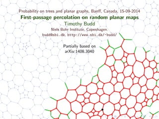
1. Probability on trees and planar graphs, Banff, Canada, 15-09-2014
First-passage percolation on random planar maps
Timothy Budd
Niels Bohr Institute, Copenhagen.
budd@nbi.dk, http://www.nbi.dk/~budd/
Partially based on
arXiv:1408.3040

2. First-passage percolation on a graph
Random i.i.d. edge weights w(e)
with mean 1.
Passage time v1 → v2
T = min
γ:v1→v2
e∈γ
w(e)

3. First-passage percolation on a graph
Random i.i.d. edge weights w(e)
with mean 1.
Passage time v1 → v2
T = min
γ:v1→v2
e∈γ
w(e)

4. First-passage percolation on a graph
Random i.i.d. edge weights w(e)
with mean 1.
Passage time v1 → v2
T = min
γ:v1→v2
e∈γ
w(e)

5. First-passage percolation on a graph
Random i.i.d. edge weights w(e)
with mean 1.
Passage time v1 → v2
T = min
γ:v1→v2
e∈γ
w(e)

6. First-passage percolation on a graph
Random i.i.d. edge weights w(e)
with mean 1.
Passage time v1 → v2
T = min
γ:v1→v2
e∈γ
w(e)

7. First-passage percolation on a graph
Random i.i.d. edge weights w(e)
with mean 1.
Passage time v1 → v2
T = min
γ:v1→v2
e∈γ
w(e)

8. First-passage percolation on a graph
Random i.i.d. edge weights w(e)
with mean 1.
Passage time v1 → v2
T = min
γ:v1→v2
e∈γ
w(e)

9. First-passage percolation on a graph
Random i.i.d. edge weights w(e)
with mean 1.
Passage time v1 → v2
T = min
γ:v1→v2
e∈γ
w(e)
Exponential distribution: equivalent
to an Eden model.

10. First-passage percolation on a graph
Random i.i.d. edge weights w(e)
with mean 1.
Passage time v1 → v2
T = min
γ:v1→v2
e∈γ
w(e)
Exponential distribution: equivalent
to an Eden model.

11. First-passage percolation on a graph
Random i.i.d. edge weights w(e)
with mean 1.
Passage time v1 → v2
T = min
γ:v1→v2
e∈γ
w(e)
Exponential distribution: equivalent
to an Eden model.

12. First-passage percolation on a graph
Random i.i.d. edge weights w(e)
with mean 1.
Passage time v1 → v2
T = min
γ:v1→v2
e∈γ
w(e)
Exponential distribution: equivalent
to an Eden model.

13. First-passage percolation on a graph
Random i.i.d. edge weights w(e)
with mean 1.
Passage time v1 → v2
T = min
γ:v1→v2
e∈γ
w(e)
Exponential distribution: equivalent
to an Eden model.

14. First-passage percolation on a graph
Random i.i.d. edge weights w(e)
with mean 1.
Passage time v1 → v2
T = min
γ:v1→v2
e∈γ
w(e)
Exponential distribution: equivalent
to an Eden model.

15. First-passage percolation on a graph
Random i.i.d. edge weights w(e)
with mean 1.
Passage time v1 → v2
T = min
γ:v1→v2
e∈γ
w(e)
Exponential distribution: equivalent
to an Eden model.

16. First-passage percolation on a graph
Random i.i.d. edge weights w(e)
with mean 1.
Passage time v1 → v2
T = min
γ:v1→v2
e∈γ
w(e)
Exponential distribution: equivalent
to an Eden model.
How does T compare to the graph
distance d (asymptotically)?

17. First-passage percolation on a graph
Random i.i.d. edge weights w(e)
with mean 1.
Passage time v1 → v2
T = min
γ:v1→v2
e∈γ
w(e)
Exponential distribution: equivalent
to an Eden model.
How does T compare to the graph
distance d (asymptotically)?
Hop count h is the number of
edges in shortest time path.

18. First-passage percolation on a graph
Random i.i.d. edge weights w(e)
with mean 1.
Passage time v1 → v2
T = min
γ:v1→v2
e∈γ
w(e)
Exponential distribution: equivalent
to an Eden model.
How does T compare to the graph
distance d (asymptotically)?
Hop count h is the number of
edges in shortest time path.
Asymptotically T < d < h.

19. Time constants
For many plane graphs (Z2
, Poisson-Voronoi, Random Geometric)
one can show that the time constants limd→∞ T/d and limd→∞ h/d
exist almost surely using Kingman’s subadditive ergodic theorem.

20. Time constants
For many plane graphs (Z2
, Poisson-Voronoi, Random Geometric)
one can show that the time constants limd→∞ T/d and limd→∞ h/d
exist almost surely using Kingman’s subadditive ergodic theorem.
However, very few exact time constants known (ladder graph,. . . ?).

21. Time constants
For many plane graphs (Z2
, Poisson-Voronoi, Random Geometric)
one can show that the time constants limd→∞ T/d and limd→∞ h/d
exist almost surely using Kingman’s subadditive ergodic theorem.
However, very few exact time constants known (ladder graph,. . . ?).
Numerically, many models seem to have d right in the middle of the
bounds (T < d < h). Explanation?

22. Time constants
For many plane graphs (Z2
, Poisson-Voronoi, Random Geometric)
one can show that the time constants limd→∞ T/d and limd→∞ h/d
exist almost surely using Kingman’s subadditive ergodic theorem.
However, very few exact time constants known (ladder graph,. . . ?).
Numerically, many models seem to have d right in the middle of the
bounds (T < d < h). Explanation?

23. Time constants
For many plane graphs (Z2
, Poisson-Voronoi, Random Geometric)
one can show that the time constants limd→∞ T/d and limd→∞ h/d
exist almost surely using Kingman’s subadditive ergodic theorem.
However, very few exact time constants known (ladder graph,. . . ?).
Numerically, many models seem to have d right in the middle of the
bounds (T < d < h). Explanation?
Let us look at random planar maps: assuming existence of the time
constants we can compute them!

24. Multi-point functions of general planar maps
FPP on a random cubic map with exponentially distributed edge
weights shows up as a by-product of the study of distances on a
random general planar map.

25. Multi-point functions of general planar maps
FPP on a random cubic map with exponentially distributed edge
weights shows up as a by-product of the study of distances on a
random general planar map.
Bijection between quadrangulations and planar maps preserving
distance. [Miermont, ’09] [Ambjorn,TB, ’13]

26. Multi-point functions of general planar maps
FPP on a random cubic map with exponentially distributed edge
weights shows up as a by-product of the study of distances on a
random general planar map.
Bijection between quadrangulations and planar maps preserving
distance. [Miermont, ’09] [Ambjorn,TB, ’13]
Random planar map with E edges converges to Brownian map as
E → ∞. [Bettinelli,Jacob,Miermont,’13]

27. Multi-point functions of general planar maps
FPP on a random cubic map with exponentially distributed edge
weights shows up as a by-product of the study of distances on a
random general planar map.
Bijection between quadrangulations and planar maps preserving
distance. [Miermont, ’09] [Ambjorn,TB, ’13]
Random planar map with E edges converges to Brownian map as
E → ∞. [Bettinelli,Jacob,Miermont,’13]
Also allowed to derive various distance statistics, while controlling
both the number E of edges and the number F of faces:
Two-point function (rooted) [Ambjorn, TB, ’13]

28. Multi-point functions of general planar maps
FPP on a random cubic map with exponentially distributed edge
weights shows up as a by-product of the study of distances on a
random general planar map.
Bijection between quadrangulations and planar maps preserving
distance. [Miermont, ’09] [Ambjorn,TB, ’13]
Random planar map with E edges converges to Brownian map as
E → ∞. [Bettinelli,Jacob,Miermont,’13]
Also allowed to derive various distance statistics, while controlling
both the number E of edges and the number F of faces:
Two-point function (rooted) [Ambjorn, TB, ’13]
Two-point function (unrooted) [Bouttier, Fusy, Guitter, ’13]

29. Multi-point functions of general planar maps
FPP on a random cubic map with exponentially distributed edge
weights shows up as a by-product of the study of distances on a
random general planar map.
Bijection between quadrangulations and planar maps preserving
distance. [Miermont, ’09] [Ambjorn,TB, ’13]
Random planar map with E edges converges to Brownian map as
E → ∞. [Bettinelli,Jacob,Miermont,’13]
Also allowed to derive various distance statistics, while controlling
both the number E of edges and the number F of faces:
Two-point function (rooted) [Ambjorn, TB, ’13]
Two-point function (unrooted) [Bouttier, Fusy, Guitter, ’13]
Three-point function [Fusy, Guitter, ’14]

30. Multi-point functions of general planar maps
FPP on a random cubic map with exponentially distributed edge
weights shows up as a by-product of the study of distances on a
random general planar map.
Bijection between quadrangulations and planar maps preserving
distance. [Miermont, ’09] [Ambjorn,TB, ’13]
Random planar map with E edges converges to Brownian map as
E → ∞. [Bettinelli,Jacob,Miermont,’13]
Also allowed to derive various distance statistics, while controlling
both the number E of edges and the number F of faces:
Two-point function (rooted) [Ambjorn, TB, ’13]
Two-point function (unrooted) [Bouttier, Fusy, Guitter, ’13]
Three-point function [Fusy, Guitter, ’14]
Consider the limit E → ∞ keeping F fixed. In terms of . . .
. . . quadrangulation: Generalized Causal Dynamical Triangulations
(GCDT)
. . . general planar maps: after “removal of trees” cubic maps with
edges of random length.

31. From general maps to weighted cubic maps
Take a planar map with marked vertices and weight x per edge.

32. From general maps to weighted cubic maps
Take a planar map with marked vertices and weight x per edge.
Remove dangling edges
.

33. From general maps to weighted cubic maps
Take a planar map with marked vertices and weight x per edge.
Remove dangling edges and combine neighboring edges while
keeping track of length.

34. From general maps to weighted cubic maps
Take a planar map with marked vertices and weight x per edge.
Remove dangling edges and combine neighboring edges while
keeping track of length.

35. From general maps to weighted cubic maps
Take a planar map with marked vertices and weight x per edge.
Remove dangling edges and combine neighboring edges while
keeping track of length.
Each “subedge” comes with weight x((1 −
√
1 − 4x)/x)2
, hence
length is geometrically distributed.

36. From general maps to weighted cubic maps
Take a planar map with marked vertices and weight x per edge.
Remove dangling edges and combine neighboring edges while
keeping track of length.
Each “subedge” comes with weight x((1 −
√
1 − 4x)/x)2
, hence
length is geometrically distributed.
Scaling limit x → 1/4 and edge lengths (x) :=
√
4 − 16x: lengths
are exponentially distributed with mean 1. Maximal number of edges
preferred: almost surely cubic and univalent marked vertices.

37. Two-point function
2-point function for general planar maps with weight x per edge and
z per face and distance t between marked vertices: [Bouttier et al, ’13]
Gz,x (t) = log
(1 − a σt+1
)3
(1 − a σt+2)3
(1 − a σt+3
)
(1 − a σt)
, (1)
where a = a(z, x) and σ = σ(z, x) solution of algebraic equations.

38. Two-point function
2-point function for general planar maps with weight x per edge and
z per face and distance t between marked vertices: [Bouttier et al, ’13]
Gz,x (t) = log
(1 − a σt+1
)3
(1 − a σt+2)3
(1 − a σt+3
)
(1 − a σt)
, (1)
where a = a(z, x) and σ = σ(z, x) solution of algebraic equations.
Scaling z = (x)3
g, t = T/ (x), x → 1/4:
G
(1,1)
g,2 (T) = ∂3
T log(Σ cosh ΣT + α sinh ΣT), Σ := 3
2 α2 − 1
8 ,
and α is solution to α3
− α/4 + g = 0.

39. Two-point function
2-point function for general planar maps with weight x per edge and
z per face and distance t between marked vertices: [Bouttier et al, ’13]
Gz,x (t) = log
(1 − a σt+1
)3
(1 − a σt+2)3
(1 − a σt+3
)
(1 − a σt)
, (1)
where a = a(z, x) and σ = σ(z, x) solution of algebraic equations.
Scaling z = (x)3
g, t = T/ (x), x → 1/4:
G
(1,1)
g,2 (T) = ∂3
T log(Σ cosh ΣT + α sinh ΣT), Σ := 3
2 α2 − 1
8 ,
and α is solution to α3
− α/4 + g = 0.
Bivalent marked vertices:
G
(2,2)
g,2 (T) = 1
4 (1 + ∂T )2
G
(1,1)
g,2 (T)

40. Two-point function
2-point function for general planar maps with weight x per edge and
z per face and distance t between marked vertices: [Bouttier et al, ’13]
Gz,x (t) = log
(1 − a σt+1
)3
(1 − a σt+2)3
(1 − a σt+3
)
(1 − a σt)
, (1)
where a = a(z, x) and σ = σ(z, x) solution of algebraic equations.
Scaling z = (x)3
g, t = T/ (x), x → 1/4:
G
(1,1)
g,2 (T) = ∂3
T log(Σ cosh ΣT + α sinh ΣT), Σ := 3
2 α2 − 1
8 ,
and α is solution to α3
− α/4 + g = 0.
Bivalent marked vertices:
G
(2,2)
g,2 (T) = 1
4 (1 + ∂T )2
G
(1,1)
g,2 (T)
Completely cubic:
G
(3,3)
g,2 (T) = 1
9 (2 + ∂T )2
G
(2,2)
g,2 (T)

41. Two-point function
2-point function for general planar maps with weight x per edge and
z per face and distance t between marked vertices: [Bouttier et al, ’13]
Gz,x (t) = log
(1 − a σt+1
)3
(1 − a σt+2)3
(1 − a σt+3
)
(1 − a σt)
, (1)
where a = a(z, x) and σ = σ(z, x) solution of algebraic equations.
Scaling z = (x)3
g, t = T/ (x), x → 1/4:
G
(1,1)
g,2 (T) = ∂3
T log(Σ cosh ΣT + α sinh ΣT), Σ := 3
2 α2 − 1
8 ,
and α is solution to α3
− α/4 + g = 0.
Scaling limit: g → 1
12
√
3
, i.e.
α → 1√
12
and Σ → 0.
Renormalizing T := ΣT gives
G
(1,1)
g,2 (T)Σ−3
→ 2
cosh T
sinh3
T
.

42. Two-point function
2-point function for general planar maps with weight x per edge and
z per face and distance t between marked vertices: [Bouttier et al, ’13]
Gz,x (t) = log
(1 − a σt+1
)3
(1 − a σt+2)3
(1 − a σt+3
)
(1 − a σt)
, (1)
where a = a(z, x) and σ = σ(z, x) solution of algebraic equations.
Scaling z = (x)3
g, t = T/ (x), x → 1/4:
G
(1,1)
g,2 (T) = ∂3
T log(Σ cosh ΣT + α sinh ΣT), Σ := 3
2 α2 − 1
8 ,
and α is solution to α3
− α/4 + g = 0.
Scaling limit: g → 1
12
√
3
, i.e.
α → 1√
12
and Σ → 0.
Renormalizing T := ΣT gives
G
(1,1)
g,2 (T)Σ−3
→ 2
cosh T
sinh3
T
.
Agrees with distance-profile of the
Brownian map.

43. Three-point function
Three marked vertices with pair-wise distances d12, d13 and d23.

44. Three-point function
Three marked vertices with pair-wise distances d12, d13 and d23.

45. Three-point function
Three marked vertices with pair-wise distances d12, d13 and d23.

46. Three-point function
Three marked vertices with pair-wise distances d12, d13 and d23.
Reparametrize d12 = s + t, d13 = s + u, d23 = u + t.

47. Three-point function
Three marked vertices with pair-wise distances d12, d13 and d23.
Reparametrize d12 = s + t, d13 = s + u, d23 = u + t.
Even case: s, t, u ∈ Z. Odd case: s, t, u ∈ Z + 1
2 .

48. Three-point function
Three marked vertices with pair-wise distances d12, d13 and d23.
Reparametrize d12 = s + t, d13 = s + u, d23 = u + t.
Even case: s, t, u ∈ Z. Odd case: s, t, u ∈ Z + 1
2 .

49. Three-point function
Three marked vertices with pair-wise distances d12, d13 and d23.
Reparametrize d12 = s + t, d13 = s + u, d23 = u + t.
Even case: s, t, u ∈ Z. Odd case: s, t, u ∈ Z + 1
2 .
Explicit expressions Geven
z,x (s, t, u), Godd
z,x (s, t, u) known. [Fusy, Guitter,
’14]

50. Three-point function
Three marked vertices with pair-wise distances d12, d13 and d23.
Reparametrize d12 = s + t, d13 = s + u, d23 = u + t.
Even case: s, t, u ∈ Z. Odd case: s, t, u ∈ Z + 1
2 .
Explicit expressions Geven
z,x (s, t, u), Godd
z,x (s, t, u) known. [Fusy, Guitter,
’14]
Scaling as before: G
(1)
g,3(S, T, U) = Geven
g,3 (S, T, U) + Godd
g,3 (S, T, U).

51. Three-point function
Three marked vertices with pair-wise distances d12, d13 and d23.
Reparametrize d12 = s + t, d13 = s + u, d23 = u + t.
Even case: s, t, u ∈ Z. Odd case: s, t, u ∈ Z + 1
2 .
Explicit expressions Geven
z,x (s, t, u), Godd
z,x (s, t, u) known. [Fusy, Guitter,
’14]
Scaling as before: G
(1)
g,3(S, T, U) = Geven
g,3 (S, T, U) + Godd
g,3 (S, T, U).
Scaling again g → 1
12
√
3
, T := ΣT, etc., gives
G
(1)
g,3(S, T, U)Σ−2
→ 1
12 ∂S∂T ∂U
sinh2
S sinh2
T sinh2
U sinh2
(S + T + U)
sinh2
(S + T ) sinh2
(T + U) sinh2
(U + S)
,
which is the Brownian map 3-point function.

52. Three-point function
Three marked vertices with pair-wise distances d12, d13 and d23.
Reparametrize d12 = s + t, d13 = s + u, d23 = u + t.
Even case: s, t, u ∈ Z. Odd case: s, t, u ∈ Z + 1
2 .
Explicit expressions Geven
z,x (s, t, u), Godd
z,x (s, t, u) known. [Fusy, Guitter,
’14]
Scaling as before: G
(1)
g,3(S, T, U) = Geven
g,3 (S, T, U) + Godd
g,3 (S, T, U).
Unless cycle vanishes, i.e.
completely confluent, even and odd
occur with equal probability. Hence
Gconf
g,3 = Geven
g,3 − Godd
g,3

53. Three-point function
Three marked vertices with pair-wise distances d12, d13 and d23.
Reparametrize d12 = s + t, d13 = s + u, d23 = u + t.
Even case: s, t, u ∈ Z. Odd case: s, t, u ∈ Z + 1
2 .
Explicit expressions Geven
z,x (s, t, u), Godd
z,x (s, t, u) known. [Fusy, Guitter,
’14]
Scaling as before: G
(1)
g,3(S, T, U) = Geven
g,3 (S, T, U) + Godd
g,3 (S, T, U).
Unless cycle vanishes, i.e.
completely confluent, even and odd
occur with equal probability. Hence
Gconf
g,3 = Geven
g,3 − Godd
g,3

54. Three-point function
Three marked vertices with pair-wise distances d12, d13 and d23.
Reparametrize d12 = s + t, d13 = s + u, d23 = u + t.
Even case: s, t, u ∈ Z. Odd case: s, t, u ∈ Z + 1
2 .
Explicit expressions Geven
z,x (s, t, u), Godd
z,x (s, t, u) known. [Fusy, Guitter,
’14]
Scaling as before: G
(1)
g,3(S, T, U) = Geven
g,3 (S, T, U) + Godd
g,3 (S, T, U).
Unless cycle vanishes, i.e.
completely confluent, even and odd
occur with equal probability. Hence
Gconf
g,3 = Geven
g,3 − Godd
g,3
Bivalent marked vertices
G
(2)
g,3 =1
8 (1 + ∂S )(1 + ∂T )(1 + ∂U )G
(1)
g,3(S, T, U)
+ G
(2)
g,2(T + U)δ(S) + G
(2)
g,2(U + S)δ(T) + G
(2)
g,2(S + T)δ(U)

55. Three-point function
Three marked vertices with pair-wise distances d12, d13 and d23.
Reparametrize d12 = s + t, d13 = s + u, d23 = u + t.
Even case: s, t, u ∈ Z. Odd case: s, t, u ∈ Z + 1
2 .
Explicit expressions Geven
z,x (s, t, u), Godd
z,x (s, t, u) known. [Fusy, Guitter,
’14]
Scaling as before: G
(1)
g,3(S, T, U) = Geven
g,3 (S, T, U) + Godd
g,3 (S, T, U).
Unless cycle vanishes, i.e.
completely confluent, even and odd
occur with equal probability. Hence
Gconf
g,3 = Geven
g,3 − Godd
g,3
Bivalent marked vertices
G
(2)
g,3 =1
8 (1 + ∂S )(1 + ∂T )(1 + ∂U )G
(1)
g,3(S, T, U)
+ G
(2)
g,2(T + U)δ(S) + G
(2)
g,2(U + S)δ(T) + G
(2)
g,2(S + T)δ(U)

56. Expected hop count for random cubic map
Consider the limit T → 0 (but S, T, U > 0) of the completely
confluent three-point function, i.e.
ˆG
(2)
g,2(S, U) := lim
T→0
1
8 (1+∂S )(1+∂T )(1+∂U )[Geven
g,3 (S, T, U)−Godd
g,3 (S, T, U)]

57. Expected hop count for random cubic map
Consider the limit T → 0 (but S, T, U > 0) of the completely
confluent three-point function, i.e.
ˆG
(2)
g,2(S, U) := lim
T→0
1
8 (1+∂S )(1+∂T )(1+∂U )[Geven
g,3 (S, T, U)−Godd
g,3 (S, T, U)]

58. Expected hop count for random cubic map
Consider the limit T → 0 (but S, T, U > 0) of the completely
confluent three-point function, i.e.
ˆG
(2)
g,2(S, U) := lim
T→0
1
8 (1+∂S )(1+∂T )(1+∂U )[Geven
g,3 (S, T, U)−Godd
g,3 (S, T, U)]

59. Expected hop count for random cubic map
Consider the limit T → 0 (but S, T, U > 0) of the completely
confluent three-point function, i.e.
ˆG
(2)
g,2(S, U) := lim
T→0
1
8 (1+∂S )(1+∂T )(1+∂U )[Geven
g,3 (S, T, U)−Godd
g,3 (S, T, U)]
Hence, for fixed number of faces F,
ˆG
(2)
F,2(S, T − S)
G
(2)
F,2(T)
is the expected density of vertices
(at distance S) along a geodesic of
length/passage time T.

60. Expected hop count for random cubic map
Consider the limit T → 0 (but S, T, U > 0) of the completely
confluent three-point function, i.e.
ˆG
(2)
g,2(S, U) := lim
T→0
1
8 (1+∂S )(1+∂T )(1+∂U )[Geven
g,3 (S, T, U)−Godd
g,3 (S, T, U)]
Hence, for fixed number of faces F,
ˆG
(2)
F,2(S, T − S)
G
(2)
F,2(T)
is the expected density of vertices
(at distance S) along a geodesic of
length/passage time T.
Scaling limit:
ˆG
(2)
g,2(S, T −S) → (1+ 1√
3
)G
(2)
g,2(T).

61. Expected hop count for random cubic map
Consider the limit T → 0 (but S, T, U > 0) of the completely
confluent three-point function, i.e.
ˆG
(2)
g,2(S, U) := lim
T→0
1
8 (1+∂S )(1+∂T )(1+∂U )[Geven
g,3 (S, T, U)−Godd
g,3 (S, T, U)]
Hence, for fixed number of faces F,
ˆG
(2)
F,2(S, T − S)
G
(2)
F,2(T)
is the expected density of vertices
(at distance S) along a geodesic of
length/passage time T.
Scaling limit:
ˆG
(2)
g,2(S, T −S) → (1+ 1√
3
)G
(2)
g,2(T).
Asymptotic hop count to passage time ratio is h /T → 1 + 1√
3
.

62. Time constants for FPP on a random cubic graph
We have seen h /T → 1 + 1√
3
. This is confirmed numerically
(random triangulation 128k triangles).

63. Time constants for FPP on a random cubic graph
We have seen h /T → 1 + 1√
3
. This is confirmed numerically
(random triangulation 128k triangles).
Let us assume that h, T and the graph distance d are
asymptotically (almost surely) linearly related.

64. Time constants for FPP on a random cubic graph
We have seen h /T → 1 + 1√
3
. This is confirmed numerically
(random triangulation 128k triangles).
Let us assume that h, T and the graph distance d are
asymptotically (almost surely) linearly related.
Then we can determine the ratio d/T simply by comparing the
corresponding two-point functions.

65. Time constants for FPP on a random cubic graph
We have seen h /T → 1 + 1√
3
. This is confirmed numerically
(random triangulation 128k triangles).
Let us assume that h, T and the graph distance d are
asymptotically (almost surely) linearly related.
Then we can determine the ratio d/T simply by comparing the
corresponding two-point functions.
Deduce from transfer matrix approach in [Kawai et al, ’93]:
h/T → 1 + 1
2
√
3
.

66. Time constants for FPP on a random cubic graph
We have seen h /T → 1 + 1√
3
. This is confirmed numerically
(random triangulation 128k triangles).
Let us assume that h, T and the graph distance d are
asymptotically (almost surely) linearly related.
Then we can determine the ratio d/T simply by comparing the
corresponding two-point functions.
Deduce from transfer matrix approach in [Kawai et al, ’93]:
h/T → 1 + 1
2
√
3
.
Simple relation: d = (h + T)/2. Is it true more generally?

67. Expected hop count for p-regular maps
Two vertices a distance T apart.

68. Expected hop count for p-regular maps
Two vertices a distance T apart.

69. Expected hop count for p-regular maps
Two vertices a distance T apart.
Determine the balls of radius S and
T − S − δS. They almost touch.

70. Expected hop count for p-regular maps
Two vertices a distance T apart.
Determine the balls of radius S and
T − S − δS. They almost touch.

71. Expected hop count for p-regular maps
Two vertices a distance T apart.
Determine the balls of radius S and
T − S − δS. They almost touch.

72. Expected hop count for p-regular maps
Two vertices a distance T apart.
Determine the balls of radius S and
T − S − δS. They almost touch.

73. Expected hop count for p-regular maps
Two vertices a distance T apart.
Determine the balls of radius S and
T − S − δS. They almost touch.
As δS → 0, conditioned on the balls, a
vertex occurs with probability P δS with
P = (p−1)
WN−1,d+p−2
WN,d
in terms of the disk function
Wx (z) =
∞
N=0
∞
d=1 z−d−1
xN
WN,d .

74. Expected hop count for p-regular maps
Two vertices a distance T apart.
Determine the balls of radius S and
T − S − δS. They almost touch.
As δS → 0, conditioned on the balls, a
vertex occurs with probability P δS with
P = (p−1)
WN−1,d+p−2
WN,d
in terms of the disk function
Wx (z) =
∞
N=0
∞
d=1 z−d−1
xN
WN,d .

75. Expected hop count for p-regular maps
Two vertices a distance T apart.
Determine the balls of radius S and
T − S − δS. They almost touch.
As δS → 0, conditioned on the balls, a
vertex occurs with probability P δS with
P = (p−1)
WN−1,d+p−2
WN,d
in terms of the disk function
Wx (z) =
∞
N=0
∞
d=1 z−d−1
xN
WN,d .

76. Expected hop count for p-regular maps
Two vertices a distance T apart.
Determine the balls of radius S and
T − S − δS. They almost touch.
As δS → 0, conditioned on the balls, a
vertex occurs with probability P δS with
P = (p−1)
WN−1,d+p−2
WN,d
→
N,d→∞
(p−1)xc zp−2
c ,
in terms of the disk function
Wx (z) =
∞
N=0
∞
d=1 z−d−1
xN
WN,d .

77. Expected hop count for p-regular maps
Two vertices a distance T apart.
Determine the balls of radius S and
T − S − δS. They almost touch.
As δS → 0, conditioned on the balls, a
vertex occurs with probability P δS with
P = (p−1)
WN−1,d+p−2
WN,d
→
N,d→∞
(p−1)xc zp−2
c ,
in terms of the disk function
Wx (z) =
∞
N=0
∞
d=1 z−d−1
xN
WN,d .
Asymptotic hop count to passage time ratio is h /T → (p − 1)xc zp−2
c .

78. Expected hop count for p-regular maps
Two vertices a distance T apart.
Determine the balls of radius S and
T − S − δS. They almost touch.
As δS → 0, conditioned on the balls, a
vertex occurs with probability P δS with
P = (p−1)
WN−1,d+p−2
WN,d
→
N,d→∞
(p−1)xc zp−2
c ,
in terms of the disk function
Wx (z) =
∞
N=0
∞
d=1 z−d−1
xN
WN,d .
Asymptotic hop count to passage time ratio is h /T → (p − 1)xc zp−2
c .
p = 3: xc = 1/(2 33/4
), zc = 33/4
(1 + 1/
√
3), h
T = 1 + 1/
√
3.

79. Expected hop count for p-regular maps
Two vertices a distance T apart.
Determine the balls of radius S and
T − S − δS. They almost touch.
As δS → 0, conditioned on the balls, a
vertex occurs with probability P δS with
P = (p−1)
WN−1,d+p−2
WN,d
→
N,d→∞
(p−1)xc zp−2
c ,
in terms of the disk function
Wx (z) =
∞
N=0
∞
d=1 z−d−1
xN
WN,d .
Asymptotic hop count to passage time ratio is h /T → (p − 1)xc zp−2
c .
p = 3: xc = 1/(2 33/4
), zc = 33/4
(1 + 1/
√
3), h
T = 1 + 1/
√
3.
p even: xc = p−2
p
p
2
4
p−2
p
p/2
−1
, zc = 4p
p−2 , h
T = 2p−2 p−2
p−2
2
−1
.

80. Transfer matrix for FPP
Take a p-regular weighted planar map
with two marked points.

81. Transfer matrix for FPP
Take a p-regular weighted planar map
with two marked points.
Identify baby universes.

82. Transfer matrix for FPP
Take a p-regular weighted planar map
with two marked points.
Identify baby universes.
Cut into small passage time intervals.

83. Transfer matrix for FPP
Take a p-regular weighted planar map
with two marked points.
Identify baby universes.
Cut into small passage time intervals.
Write Gx (z, T) := d1
z−d1−1
G
(d1,d2)
x,2 (T) and
the disk function Wx (z) := d z−d−1
G
(d)
x,1
(weight x per vertex). Then
∂
∂T Gx (z, T)= ∂
∂z ( z
A
−xzp−1
B
−2 Wx (z)
C
)Gx (z, T)

84. Transfer matrix for FPP
Take a p-regular weighted planar map
with two marked points.
Identify baby universes.
Cut into small passage time intervals.
Write Gx (z, T) := d1
z−d1−1
G
(d1,d2)
x,2 (T) and
the disk function Wx (z) := d z−d−1
G
(d)
x,1
(weight x per vertex). Then
∂
∂T Gx (z, T)= ∂
∂z ( z −xzp−1
−2Wx (z))Gx (z, T)
Precisely this formula was used in
[Ambjorn, Watabiki, ’95] as an approximation
to derive the 2-point function for
triangulations. Now we know it is not
just an approximation!

85. Transfer matrix for graph distance [Kawai et al, ’93]
Now take all edges to have length 1.
Again we can build a transfer matrix.

86. Transfer matrix for graph distance [Kawai et al, ’93]
Now take all edges to have length 1.
Again we can build a transfer matrix.

87. Transfer matrix for graph distance [Kawai et al, ’93]
Now take all edges to have length 1.
Again we can build a transfer matrix.

88. Transfer matrix for graph distance [Kawai et al, ’93]
Now take all edges to have length 1.
Again we can build a transfer matrix.
Two of the building blocks are quite
similar. . .

89. Transfer matrix for graph distance [Kawai et al, ’93]
Now take all edges to have length 1.
Again we can build a transfer matrix.
Two of the building blocks are quite
similar. . .
. . . but there are p − 1 extra ones.

90. Transfer matrix for graph distance [Kawai et al, ’93]
Now take all edges to have length 1.
Again we can build a transfer matrix.
Two of the building blocks are quite
similar. . .
. . . but there are p − 1 extra ones.
Can work out transfer matrix PDE
explicitly and compare, but heuristically
∼ ∼ xc zp−2
c

91. Transfer matrix for graph distance [Kawai et al, ’93]
Now take all edges to have length 1.
Again we can build a transfer matrix.
Two of the building blocks are quite
similar. . .
. . . but there are p − 1 extra ones.
Can work out transfer matrix PDE
explicitly and compare, but heuristically
∼ ∼ xc zp−2
c
and therefore
+ + + +
2
→ 1
2 (1 + (p − 1)xc zp−2
c )
Graph distance to passage time ratio is
d/T → (1 + h/T)/2.

92. Conclusion & open questions
Conclusions
Both the two- and three-point functions of weighted cubic maps
converge to those of the Brownian map in the scaling limit.
We can compute the time constants of FPP on random p-regular
planar maps, and in each case they satisfy d = (h + T)/2.

93. Conclusion & open questions
Conclusions
Both the two- and three-point functions of weighted cubic maps
converge to those of the Brownian map in the scaling limit.
We can compute the time constants of FPP on random p-regular
planar maps, and in each case they satisfy d = (h + T)/2.
Open questions
Can weighted cubic maps be shown to converge to the Brownian
map?

94. Conclusion & open questions
Conclusions
Both the two- and three-point functions of weighted cubic maps
converge to those of the Brownian map in the scaling limit.
We can compute the time constants of FPP on random p-regular
planar maps, and in each case they satisfy d = (h + T)/2.
Open questions
Can weighted cubic maps be shown to converge to the Brownian
map?
Is d = (h + T)/2 a coincidence or does it hold for a (much) larger
class of random graphs? Does it hold in the case of . . .
. . . weights on the faces, e.g. p-angulations?
. . . other edge length distributions?
. . . random geometric graphs (in certain limits)?

95. Conclusion & open questions
Conclusions
Both the two- and three-point functions of weighted cubic maps
converge to those of the Brownian map in the scaling limit.
We can compute the time constants of FPP on random p-regular
planar maps, and in each case they satisfy d = (h + T)/2.
Open questions
Can weighted cubic maps be shown to converge to the Brownian
map?
Is d = (h + T)/2 a coincidence or does it hold for a (much) larger
class of random graphs? Does it hold in the case of . . .
. . . weights on the faces, e.g. p-angulations?
. . . other edge length distributions?
. . . random geometric graphs (in certain limits)?
Is there a bijective explanation for d = (h + T)/2?

96. Conclusion & open questions
Conclusions
Both the two- and three-point functions of weighted cubic maps
converge to those of the Brownian map in the scaling limit.
We can compute the time constants of FPP on random p-regular
planar maps, and in each case they satisfy d = (h + T)/2.
Open questions
Can weighted cubic maps be shown to converge to the Brownian
map?
Is d = (h + T)/2 a coincidence or does it hold for a (much) larger
class of random graphs? Does it hold in the case of . . .
. . . weights on the faces, e.g. p-angulations?
. . . other edge length distributions?
. . . random geometric graphs (in certain limits)?
Is there a bijective explanation for d = (h + T)/2?
How do the relative fluctuations of d, h, T scale?
Kardar-Parisi-Zhang scaling exponents on a random surface?

97. Conclusion & open questions
Conclusions
Both the two- and three-point functions of weighted cubic maps
converge to those of the Brownian map in the scaling limit.
We can compute the time constants of FPP on random p-regular
planar maps, and in each case they satisfy d = (h + T)/2.
Open questions
Can weighted cubic maps be shown to converge to the Brownian
map?
Is d = (h + T)/2 a coincidence or does it hold for a (much) larger
class of random graphs? Does it hold in the case of . . .
. . . weights on the faces, e.g. p-angulations?
. . . other edge length distributions?
. . . random geometric graphs (in certain limits)?
Is there a bijective explanation for d = (h + T)/2?
How do the relative fluctuations of d, h, T scale?
Kardar-Parisi-Zhang scaling exponents on a random surface?
Thanks!