SlideShare a Scribd company logo
1 of 136
From First Principles June 2017 – R4.0
Maurice R. TREMBLAY
Standard Particles SUSY Particles
PART IX – SUPERSYMMETRY
Higgs Higgsino
Quarks SquarksLeptons SleptonsForce particles SUSY force
particles
Supersymmetry is a symmetry that unites particles of integer and half-integer spin in
common symmetry multiplets (e.g., a group of related subatomic particles) – it is a
symmetry connecting bosons and fermions. It is a possible symmetry of nature in four
space-time dimensions and it has the quality of uniqueness that physicists search for in
fundamental physical theories. There is an infinite number of Lie groups that can be
used to combine particles of the same spin in ordinary symmetry multiplets, but there
are only eight kinds of supersymmetry in four space-time dimensions, of which only one,
the simplest, could be directly relevant to observed particles. Unfortunately, there is still
no direct evidence for supersymmetry, as no pair of particles related to supersymmetry
transformations has yet been discovered. There is one significant piece of indirect
evidence for supersymmetry: the high-energy unification of the SU(3)C⊗SU(2)L⊗U(1)Y
gauge couplings works better with the extra particles called for by supersymmetry than
without them. Or maybe the problem might still reside with the point particle concept*.
Forward
2
2017
MRT
As with my other work, nothing of this is new or even developed first hand and frankly
it is a rearranged compilation of various quotes from various sources (c.f., References)
that aims to display an abridged but yet concise and straightforward mathematical
developmentof supersymmetry(and some higher-dimensional theories too) as I
understand it and wish it to be presented to the layman or to the inquisitive person. As a
matter of convention, I have included the setting h≡c≡1 in most of the equations and
ancillary theoretical discussions and I use the summation convention that implies the
summation over any repeated indices (typically subscript-superscript) in an equation.
* A point particle is an idealization of particles heavily used in physics. Its defining feature is that it lacks spatial extension.
Contents
2017
MRT
PART IX – SUPERSYMMETRY
Motivation
Introduction to Supersymmetry
The SUSY Algebra
Realizations of the SUSY Algebra
The Wess-Zumino Model
Lagrangian with Mass and Interaction
Terms
The Superpotential
Supersymmetric Gauge Theory
Spontaneous Breaking of
Supersymmetry
F-type SUSY Breaking
D-type SUSY Breaking
The Scale of SUSY Breaking
The SUSY Particle Spectrum
Supersymmetric Grand Unification
General Relativity
The Principle of Equivalence
General Coordinates
“Supersymmetry […] introduces, apart from the three obvious dimensions plus time, new ‘quantum’
dimensions that cannot be measured by numbers; they are ‘quantum’ (or ‘fermionic’) dimensions, like the
spin of the electron.” Edward Witten, The Quest for Supersymmetry talk at the Perimeter Institute.
Local Lorentz Frames
Local Lorentz Transformations
General Coordinate Transformations
Covariant Derivative
The Einstein Lagrangian
The Curvature Tensor
The Inclusion of Matter
The Newtonian Limit
Local Supersymmetry
A Pure SUGRA Lagrangian
Coupling SUGRA to Matter and Gauge
Fields
Higher-dimensional Theories
Compactification
The Kaluza Model of Electromagnetism
Non-Abelian Kaluza-Klein Theories
Kaluza-Klein Models and the Real World
N=1 SUGRA in Eleven Dimensions
References
The idea that there may be a symmetry called supersymmetry (SUSY) that interrelates
bosons and fermions is rather attractive. In particular, SUSY might help to solve the
hierarchy problem discussed in PART VIII – THE STANDARD MODEL: Hierarchy
Problem. We saw there that the origin of this problem is the difficulty of including
fundamental scalar Higgs fields in the theory. Scalars are the only fields that can have
nonzero vacuum expectation values (and so give spontaneous symmetry breaking)
without breaking the Lorentz invariance of a theory. On the other hand, the masses of
such scalars are subject to quadratically divergent renormalization corrections of the like
of ∆MH
2 ∝[g2/(2π)4]∫
Λ
(1/k2)d4k ~(g2/8π2)Λ2 and there is no natural way to sustain a light
Higgs of mass O(MW) together with a heavy Higgs of O(MX). There will be radiative
corrections to the light Higgs mass of O(MX) that automatically destroy the hierarchy.
Only by an unnatural fine tuning of parameters, order-by-order in perturbation theory,
could we keep a light Higgs of mass O(MW). A natural solution would be the existence of
a symmetry that requires that certain scalars must have zero mass. Chiral symmetry
ensures zero fermion masses by forbidding mass terms like mψRψL. This appears
unlikely to help with scalars because the scalar mass term, m2φφ*, always respects this
symmetry. However, in a supersymmetric model each scalar mass must be equal to that
of its fermion partner, which can be required to vanish by chiral symmetry. Moreover, the
scalar mass, MH, is then no longer quadratically divergent because the boson and
fermion loop corrections in ∆MH
2 above have opposite signs and cancel each other:
Motivation
4
2017
MRT0~~
fermion
22
boson
222
H =ΛΛ∆ ggM
_
We begin by introducing the generators of SUSY transformations, Q, which turns
fermions F into bosons B and vice versa:
5
2017
MRT
Owing to the fermionic character of Q, any supersymmetric multiplet must contain
numbers of bosons and fermions of the same mass. Nature, however, is manifestly not
supersymmetric. The known bosons and fermions do not group themselves into such
mass-degenerate pairs. (N.B., the vacuum state is labelled by |0〉 regardless).
FBBF == QQ and
Although experimental support for supersymmetry is still lacking, many people believe
(e.g., the likes of Edward Witten!) that it is too beautiful to have been discarded by
nature, and that it is only a matter of time before evidence of SUSY, albeit in some
broken form, will be found. We need a finite Higgs mass of O(MW) to produce the obser-
ved electroweak symmetry breaking, so we want to break SUSY gently so that ∆MH
2
above becomes:
)( 2
F
2
B
22
H mmgM −∝∆
So if this last equation is to give ∆MH
2 < MH
2, supersymmetric partners of the ordinary
particles must be found with masses <1 TeV.~
~
In the subsequent chapters we will give an introduction of the main ingredients of
supersymmetric theories. For further technical details of the general formalism of
SUSY, we suggest the References and note that the definitive authoritative reference
seems to be Supersymmetry and Supergravity, 2nd Ed., Wess and Bagger (1992).
Introduction to Supersymmetry
Now, to illustrate how supersymmetry works, we begin with the following example,
which includes many of the most important features of SUSY theories. Consider a
simple harmonic oscillator with both bosonic and fermionic degrees of freedom.
6
2017
MRT
0],[],[1],[],[ ††††††
===≡≡− − bbbbbbbbbbbb and
while those of the fermion (i.e., f † and f ) satisfy the anticommutation relations:
0},{},{1},{],[ ††††††
===≡≡+ + ffffffffffff and
Since f †f †|0〉=0, two fermions cannot occupy the same state (i.e., Pauli’s exclusion
principle). In terms of these operators, the Hamiltonian takes the form:
],[ω½},{ω½ †
F
†
B ffbbH +=
where ωB and ωF are the classical frequencies of the boson and fermion oscillators,
respectively, and the allowed energies are:
)(ω)½(ω)½(ω FBFFBB nnnnE +=+++=
if ωB =ωF =ω. In this supersymmetry limit we have exact cancellation of the zero-point
energies! So, nF=0,1 are the only allowed eigenvalues of the fermion number
operator, f †f, and so all the energy levels are doubly degenerate, except for the
ground state (i.e., nB =nF=0). The system thus contains equal numbers of bosonic
and fermionic degrees of freedom!
The creation and annihilation operators of the boson (i.e., b†≡bcT and b, respectively,
with † the Hermitian conjugate symbol which means that one has to transpose T the matrix
then change the imaginary elements c from i to −i) satisfy the commutation relations:
This degeneracy indicates that there must exist some (super)symmetry of the
Hamiltonian. In fact, it is easy to check that the (annihilation and creation) charge
operators*:
7
2017
MRT
bfQfbQ †††
22 ω=ω= and
commute with the Hamiltonian H=P0 (e.g., Pµ =[P0,Pi]):
0],[],[ †
== HQHQ
with √(2ω) being just a simple normalization factor (Exercise). The operators Q and Q†
clearly have the effect of replacing a fermion by a boson, and vice versa, as in Q|F〉=|B〉
and Q|B〉=|F〉 above, and so they are supersymmetry generators. Furthermore, we find
that:
HQQ 2},{ †
=
and so the algebra of Q, Q†, and H closes if we include anticommunication as well. This
anticommutator is the essence of SUSY.
* We present a tabular representation of these operators to help in the association later on or to help in memorizing this fact.
bfQfbQ †††
22 ω=ω=
Replacing a: fermion by a boson boson by a fermion
Supersymmetric
charge generators
Operators:
This is
explained in
words by:
A fermion is
destroyed, f, and a
boson is created, b†.
A boson is destroyed,
b, and a fermion is
created, f †.
√(2ω) is a
normalization
factor.
In a 1967 paper, Sidney Coleman and Jeffrey Mandula (S.C.’s former Grad student)
adopted reasonable assumptions about the finiteness of the number of particle types
below any given mass, the existence of scattering at almost all energies, and the
analyticity of the S-matrix, and used them to show that the most general Lie algebra of
symmetry operators that commute with the S-matrix, that take single-particle states into
single-particle states, and that act on multiparticle states as the direct sum of their action
on single-particle states consists of the generators Pµ and Mµν of the Poincaré group,
plus ordinary internal symmetry generators Ta that act on one-particle states with
matrices that are diagonal in and independent of both momentum and spin.
8
2017
MRT
],,[],,[],,[],,[ 321030201321123123 KKKMMMJJJMMM =≡=≡ KJ and
So, Coleman and Mandula showed that, under very general assumptions, a Lie group
that contains both Poincaré group P and an internal symmetry G must be just a direct pro-
duct of P and G. The generators of the Poincaré group are the four-momentum Pµ=[H,P],
which produces space-time translations, and the antisymmetric tensor Mµν , which
generates space(J)-time(K) rotations:
The SUSY Algebra
where the angular momentum operator J≡Jk generates space rotations about the k-axis
and K≡Kk generates Lorentz boosts along the k-axis. So if the generators of the
Coleman-Mandula theorem requires that:
0],[],[ == aa TMTP µνµ
This no-go theorem shows the impossibility of combining space-time and internal
symmetries in any but a trivial way (or else commutators such as [.,.]=1 would exist).
Yet, formulating supersymmetry escapes this ‘no-go’ theorem because, in addition to
the generators Pµ, Mµν , Ta which satisfy commutation relations, it involves fermionic
generators Q that satisfy anticommutation relations. If we call the generators with these
properties even and odd, respectively, then the SUSY algebra has the general structure:
9
2017
MRT
odd]odd,even[even}odd,odd{even]even,even[ === and,
which is called a graded Lie algebra by mathematicians.
Without further ado we now present the simplest form of SUSY algebra. We introduce
four generators Qα (α =1,…,4),which form a four-componentMajorana spinor. Majorana
spinors are the simplest possible type of spinor. They are self-conjugate (i.e., ψ c =ψ ):
T
QCQQ c
==
and hence have only half as many degrees of freedom as a Dirac spinor. (N.B., we use
for Q the same convention as the adjoint [row] Dirac spinor, ψ =ψ †γ 0). Indeed, any Dirac
spinor ψ =[ψ1 ψ2 ψ 3 ψ 4]T may be written:
)(
2
1
21 ψψψ i+=
where:
are two independent Majorana spinors that satisfy ψ i =ψ i
c.
)(
2
)(
2
1
21
cc i
ψψψψψψ −−=+= and
__
Since Qα is a spinor, it must satisfy:
10
2017
MRT
βαβµνµνα QMQ )(
2
1
],[ Σ=
where the sum over β is implicit (i.e., summation convention for repeated indices). This
relation expresses the fact that the Qα transform as a spinor under the rotations
generated by Mµν (N.B., Σµν =½i(γ µγ ν −γ νγ µ )=½i[γ µ,γ ν ], when sandwiched between
spinors, transforms as an antisymmetric tensor). The Jacobi identity of commutators:
requires that Qα must be translationally invariant:
0]],,[[]],,[[]],,[[ =++ ανµµαννµα QPPPQPPPQ
0],[ =µα PQ
It is the remaining (anti)commutation relation (c.f., [Q,Q†]=2H of the Motivation chapter):
µαβ
µ
βα γ PQQ )(2},{ =
where the sum over µ is implicit, which we shall derive later on from first principles, and
closes the algebra, that has the most interesting consequences. Clearly this {Qα ,Qβ}
anticommutator has to yield an even generator, which might be either Pµ or Mµν . But a
term of the form Σµν Mµν (sum over µν) on the right-hand side would violate a
generalized Jacobi identity involving Qα, Qβ, and Pµ and the algebra would not close.
Indeed, if we go back to the ‘no-go’ theorem and allow for anticommutators as well as
commutators, we find that the only allowed supersymmetries are those based on the
graded Lie algebra defined by [Qα ,Mµν ], [Qα ,Pµ], and {Qα ,Qβ} above.
_
_
We choose Qα to be a Majorana spinor with four independent (real) parameters, but we
could have used a Weyl spinor with two complex components equally well. In fact, we
shall find it more convenient to work with a left-handed Weyl spinor χa with a=1,2, and
the chiral representation of the Dirac matrices in which:
11
2017
MRT





−
=





=





−
=
I
I
I
I
0
0
0
0
0
0
50 γγ and,
σσσσ
σσσσ
γγγγ
The charge-conjugation matrix, C, defined by the final equation, satisfies the require-
ment:
Realizations of the SUSY Algebra






−
=





+





==
*0
*
0 2
0
Q
QQQ
σ
γ
i
CQQ c T
In this chiral representation we find:
c
RLLL C ψψψγψψ +=+= *
0
T






−
=
0
0
2
2
0
σ
σ
γ
i
i
C T
and:
Using the two-component Weyl spinor Qa, we can construct a Majorana spinor Qα as
in:
T
µµ γγ −=−
CC 1
We then look for possible SUSY representations that contain massless particles.
These should be the relevant multiplets, since the particles we observe are thought to
acquire their masses only as a result of spontaneous symmetry breaking. The procedure
we employ is to evaluate the anticommutator {Qα ,Qβ} of the The SUSY Algebra chapter
for a massless particle moving along the z-axis with Pµ =[E,0,0,E]. On substituting Q=Qc
= [Q −iσ2 Q*]T above into {Qα ,Qβ}, we find:
12
2017
MRT
E4},{0},{0},{ †
22
†
11
†
21 === QQQQQQ and,
with a=1,2, giving:
abba E )1(2},{ 3
†
σ−=QQ
We see that Q2
† and Q2 act as creation and annihilation operators, respectively, just like
f † and f in { f , f †}=1 and { f , f }={ f † , f †}= 0 of the Motivation chapter.
_
_
Now a massless particle of spin s can only have helicities λ=±s, so, starting from the
left-handed state |s,λ=−s〉, which is annihilated by Q2, only one new state can be formed
(i.e., Q2
†|s,−s〉). This describes a particle of spin s+½ and helicity −(s+½), and by virtue
of [Qα ,Pµ]=0 of the The SUSY Algebra chapter, it is also massless. Then, acting again
with Q1
† or with Q2
† gives states of zero norm by virtue of {Q1,Q2
†}=0, {Q1,Q1
†}=0, and
also {Q2 ,Q2
†}=4E above and note that Q2
†Q2
†=0 (which follows from the fermionic nature
of Q2). So the resulting massless irreducible representation consists of just two states.
Hence, the possible supersymmetric multiplets {|s,λ〉} of interest to us are:
13
2017
MRT
















½,½
2,1
0,0
½,½
gauginosfermion
bosongaugefermion
multipletgauge)(orVectormultipletChiral
To maintain CPT invariance we must add the antiparticle states that have opposite
helicity, thus giving a total of four states, |s+½, ±(s+½)〉, |s, ±s〉, in each multiplet.
All the particles in such multiplets must carry the same gauge quantum numbers. For
this reason, the known fermions (i.e., the quarks and leptons) must be partnered by
spin-0 particles (called sfermions), not spin-1 bosons. This is because the only spin-1
bosons allowed in a renormalizable theory are the gauge bosons and they have to
belong to the adjoint representation of the gauge group, but the quarks and leptons do
not. Instead, the gauge bosons are partnered by new spin-½ gauginos(spin-3/2 being
ruled out by the requirement of renormalizability).
There is of course no experimental evidence for the existence of such spin-0 sfermions
or spin-½ gauginos. The need to introduce new supersymmetric partners, rather than
interrelate the known bosons and fermions, is undoubtedly a major setback for SUSY.
14
2017
MRT
For completeness, we briefly consider also supermultiplets of particles with nonzero
mass M. In this case, in the particle’s rest frame, Pµ=[M,0,0,M], so the anticommutator
{Qα ,Qβ}=2(γ µ)αβ Pµ of the The SUSY Algebra chapter becomes:
abba Mδ2},{ †
=QQ
We see that Qa
†/√(2M) and Qa/√(2M) act as creation and annihilation operators,
respectively, for both a=1 and 2.
Starting from a spin state |s, s3〉, which is annihilated by the Qa, we can reach three
other states by the action of Q1
†, Q2
† and Q1
†Q2
† =−Q2
†Q1
†. For example, from the spin
states |½, ±½〉 we obtain:
and hence generate a SUSY multiplet consisting of one spin-0, one spin-1 and two
spin-½ particles, all of mass M.
|½, ½〉
|½, −½〉
|1, 1〉
|1, 0〉, |0, 0〉
|½, ½〉
|½, −½〉
|1, −1〉
χ1
†
χ2
†
χ1
†
χ2
†
χ2
†
χ1
†
χ2
†
χ1
†
_
In summary, supersymmetry is a symmetry that relates bosons to fermion (i.e.,
schematically a SUSY generator Q acts as Q(fermion)=boson and Q(boson)=fermion) and
so requires an equal number of fermionic and bosonic degrees of freedom.
15
2017
MRT
∫ ∂−Φ∂Φ−∂= )*(4
ψσψ µ
µ
µ
µ
ixdS
The simplest 4D system invariant under SUSY is a free theory with Weyl fermions ψα
and a complex scalar Φ, whose action is:
Now, if we consider the convention of a metric with signature [−,+,+,+] and the Weyl
spinor notation of Wess and Bagger, we have 2-component spinors with undotted and
dotted indices ψα ,ψ α , transforming in representation (½,0) and (0,½) of the Lorentz
group. A Dirac spinor contains two Weyl spinors, ΨD=(ψα ,χα ), and a Dirac mass term
reads ψ αχα +ψα χα. Some useful identities are ψχ =ψ αχα =−ψα χα =χαψα =χψ. One also
defines [σ µ
αα ]=[−I,σσσσ] and [σ µ
αα ]=[−I,−σσσσ], where I is the 2×2 identity matrix and σσσσ the
2×2 Pauli spin matrices.
⋅⋅⋅⋅
⋅⋅⋅⋅
⋅⋅⋅⋅
⋅⋅⋅⋅
⋅⋅⋅⋅ ⋅⋅⋅⋅
This system has a current which is conserved on-shell (i.e., upon use of the equations of
motion). This so-called supercurrent is:
0)*( =∂Φ∂= µ
αµα
µν
ν
µ
α ψσσ JJ with
which implies the conservation of the (super)charges:
∫∫ == 0303
αααα && JxdQJxdQ and
_
_
_
_
These charge generators have the unusual properties of being fermionic and
transforming as Weyl spinors under the Lorentz group – rather than scalars, as more
familiar symmetry generators. Also their algebra is generated by anticommutation
relations, rather than by commutators. Since both Q and Q are conserved, their
anticommutator should be a bosonic conserved quantity. The only candidate in the
space-time momentum Pµ, necessarily contracted with σ µ to have the right spinorial
structure. Indeed explicit computation leads to the (super)algebra:
16
2017
MRT
µ
µ
αααα σ PQQ && 2},{ =
with other (anti)commutators vanishing:
0],[],[},{},{ ==== µαµαβαβα PQPQQQQQ &&&
Remarkably, Qα and Qα are not generators of an internal symmetry, rather they
intertwine with the Poincaré algebra. You can compare this to the form obtained earlier:
⋅⋅⋅⋅
µαβ
µ
βα γ PQQ )(2},{ =
with:
These are similar but do not highlight the spinorial nature of the Wess and Bagger
notation (as it is widely used in the community). Since the content here is really to
show the features of supersymmetry I revert back to the original Majorana notation.






=





−
=
0
0
0
0
0
I
I
γand
σσσσ
σσσσ
γγγγ
_
_
We are now ready to consider the construction of supersymmetric field theories such as
the Wess-Zumino Model [Supergauge transformations in four dimensions, Nuclear
Physics B 70 (1): 39–50 (1974). Look up this title here: http://booksc.org] of the
massless spin-0–spin-½ multiplet, which in some way, is an alternative introduction to
SUSY. Indeed, probably the most intuitive way of introducing SUSY is to explore,
through this simple example, possible Fermi-Bose symmetries of the Lagrangian. It
could therefore equally well have been the starting point for our discussion of SUSY.
17
2017
MRT
ψγψ µ
µµ
µ
µ
µ
∂+∂∂+∂∂= iBBAA
2
1
))((
2
1
))((
2
1
L
The simplest multiplet in which to search for SUSY consists of a two-component Weyl
spinor (or equivalently a four-component Majorana spinor) together with two real scalar
fields. To be specific, we take a massless Majorana spinor field,ψ, massless scalar field,
A, and massless pseudoscalar field, B. The kinetic energy is:
The Wess-Zumino Model
with ψ =ψ †γ 0, as usual. The unfamiliar factor of ½ in the fermion term arises because ψ
is a Majorana spinor; a Dirac spinor ψ =[ψ1 ψ2 ψ3 ψ4]T is a linear combination of two
Majorana spinors (c.f., ψ =(1/√2)(ψ1+iψ2)).
The following bilinear identities are particularly useful when exploring SUSY. For any
two Majorana spinors ψ1, ψ2 we have:
1221 ψψηψψ Γ=Γ
where η=(1,2,−1,1,−1) for Γ={1,γ5 ,γµ ,γµγ5 ,Σµν}. These relations follow directly from
when we recall that Majorana spinors are self-conjugate, ψi
c=ψi.
_
To discover the Fermi-Bose symmetries of L, we make the following infinitesimal
transformations:
18
2017
MRT
ψδψψψδδ +=′→+=′→+=′→ and, BBBBAAAA
where:
where ε is a constant infinitesimal Majorana spinor that anticommutes with ψ and
commutes with A and B. So, overall, these transformations then look like:
εγγψδψγεδψεδ µ
µ
)( 55 BiAiiBA +∂−=== and,
_ _
These transformations are Lorentz-covariant but otherwise δ A and δ B are just fairly
obvious first guesses.
ψγε
ψε
5iBB
AA
+=′
+=′
and:
εγγψψ µ
µ
)( 5BiAi +∂−=′
The possibility of constructing two independent invariant quantities εψ and εγ5ψ and ψ
have mass dimensions 1 and 3/2, respectively, ε must have dimension −½. Hence, the
derivative in δψ is therefore required to match these dimensions.
We have also assumed that the transformations have to be linear in the fields.
Under the transformations δ A=εψ, δ B=iεγ5ψ, and δψ =−iγ µ∂µ(A+iγ5B)ε above the
change in L can be written in the form:
19
2017
MRT
where we have used the identities:






+∂/∂=












+∂−+∂∂=
+∂∂+∂+∂−∂∂+∂∂=
∂+∂+∂∂+∂∂=
∂+∂+∂∂+∂∂+∂∂+∂∂=
∂+∂+∂+∂∂+∂∂+∂∂+∂∂=
∂+∂∂+∂∂=
ψγγε
ψγγγγε
εγγγψψγγγεψγεψε
ψδγψψγψδδδ
ψδγψψγψδδδδδ
ψδγψψγδψψγψδδδδδ
ψγψδδδδ
µ
µ
ν
µνµ
µ
ν
ν
µ
µ
µν
µν
µ
µ
µ
µ
µ
µ
µ
µ
µ
µ
µ
µ
µ
µ
µ
µµ
µ
µ
µ
µ
µ
µ
µ
µ
µ
µ
µ
µ
µµ
µ
µ
µ
µ
µ
µ
µ
µ
µµ
µ
µ
µ
)]([
2
1
)(
2
1
)(
])([
2
1
)(
2
1
)(
2
1
)(
2
1
)()(
)]()[(
2
1
)]()([
2
1
)]()([
2
1
)]()()([
2
1
)]()([
2
1
)]()([
2
1
)(
2
1
)(
2
1
)(
2
1
5
55
555
BiA
BiABiA
BiABiABiA
iiBBAA
iBBBBAAAA
iBBBBAAAA
iBBAAL
εγψψγεεψψε 55
== and
of ψ1Γψ2 =ηψ2Γψ1 above where η=(1,2,−1,1,−1) for Γ={1,γ5,γµ,γµγ5,Σµν}. Since δ L
is a total derivative, it integrates to zero when we form the action. Hence, the action
is invariant under the combined global supersymmetric transformations δ A=εψ, δ B=
iεγ5ψ, and δψ =−iγ µ∂µ(A+iγ5B)ε that mix the fermion and boson fields. As usual,
global is used to indicate that ε is independent of space-time (also termed rigid).
__
__
_
_
We have remarked that the δψ transformation (i.e., −iγ µ∂µ(A+iγ5B)ε) contains a
derivative. It thus relates the Fermi-Bose symmetry to the Poincaré group. In particular,
the appearance of the time derivative (i.e., ∂µ≡∂/∂xµ =[∂/∂t,∇∇∇∇]) gives an absolute
significance to the total energy, which is normally absent in theories that do not involve
gravity. This could be relevant to the value of the cosmological constant Λ.
20
2017
MRT
When we extend the global supersymmetry of this chapter to local supersymmetry, the
presence of derivatives in the algebra will imply that derivatives at different points of
space-time are related. This has the implications for the metric of space-time and will
take us into the domain of general relativity. We shall find that when we come to
construct Lagrangians that are supersymmetric under local supersymmetry
transformations we shall be forced to introduce a spin-2 particle that can be identified
with the graviton. Thus, gravity naturally and automatically becomes unified with the
other forces of physics, which is why local supersymmetry is called supergravity
(SUGRA). This enhances the interest of super theories.
It is quite amazing that spin-2 particles (but none higher!) are naturally introduced by
these limited requirements of Fermion-Boson statistics, anticommutator-commutator
graded Lie algebras, and space-time locality. These very convincing arguments are used
to explain the rationale suggesting that nature was supersymmetric in its origin and that
what we see today is just the condensation of particle states (because the universe is so
cold!) and that spontaneous symmetry breaking occurred often in the past. Of course,
the mechanisms inherently used by particle interactions and the continuous and per-
sisting issue of finding a true universal vacuum occupies most of physics even today!
Returning our attention again to the global transformations δ A=εψ, δ B=iεγ5ψ, and δψ
=−iγ µ∂µ(A+iγ5B)ε above, we recall that the commutator of two successive
transformations of a symmetry group must itself be a symmetry transformation. In this
way we identified the algebra of the generators of the group. To obtain the
corresponding result for supersymmetry, we must therefore consider two successive
SUSY transformations like δ A, δ B, and δψ. For example, if for the scalar field A we
make a transformation δ A=εψ associated with parameter ε1, followed by another with
parameter ε2, then we obtain from δψ =−iγ µ∂µ(A+iγ5B)ε:
21
2017
MRT
2511212 )()()( εγγεψεδδδ µ
µ
BiAA +∂−==
Hence, the commutator:
AP
AiAi
BiAiBiAiAA
µ
µ
µ
µ
µ
µ
µ
µ
µ
µ
εγε
εγεεγε
εγγεεγγεδδδδδδ
21
2121
152251122112
2
)(22
)()(],[)(
−=
∂−=∂−=
+∂++∂−==−
since the terms involving B cancel when we use identities for Majorana spinors (i.e., the
ψ1Γψ2 =ηψ2Γψ1 relation above where η=(1,2,−1,1,−1) for Γ={1,γ5,γµ,γµγ5,Σµν }) and, of
course, i∂µ=Pµ.
_ _
_
__
Now the generator of SUSY transformations Qα is a four-component Majorana spinor,
which we define by the requirement that (c.f., φ →exp(iα)φ ≈(1+iα)φ ≡φ +δφ and φ*→
exp(−iα)φ*≈(1−iα)φ*≡φ* +δφ*):
22
2017
MRT
AQA εδ =
To make this consistent with [δ2 ,δ1]A=−2ε1γ µε2 Pµ A above, we form the commutator:
AQQ
AQQQQ
AQQ
AQQA
},{
)(
],[
],[],[
21
2112
12
1212
βαβα
ββααααββ
εε
εεεε
εε
εεδδ
=
−=
=
=
using εψ =ψε and ε γ 5ψ =ψγ 5ε. Writing [δ2 ,δ1]A= −2ε1γ µε2 Pµ A in component form and
equating it with the last commutator, [δ2 ,δ1]A=−ε1α ε2β {Qα ,Qβ}A, reveals the basic
SUSY requirement:
µαβ
µ
βα γ PQQ )(2},{ =
which is indeed part of SUSY algebra {Qα ,Qβ} obtained earlier in the Motivation
chapter.
_
_ _
_
_ _
_
_
_
Without going into detail, the algebra closes when acting on the spinor field ψ :
23
22
aux
2
1
2
1
GFL +=
However, there is a problem with [δ2 ,δ1]ψ =−2iε1γ µε2 ∂µψ +iε1γ νε2 γν ∂ψ above
because it gives the required closure only when ψ satisfies the free Dirac equation, but
not for interacting fermions that are off the mass shell. The reason is that for off-mass-
shell particles the number of fermions and boson degrees of freedom no longer match
up. A and B still have two bosonic degrees of freedom, whereas the Majorana spinor ψ
has four. We can restore the symmetry by adding two extra bosonic fields, F and G
(called auxiliary fields because it appears without derivatives in the action hence no
dynamics associated to them), whose free Lagrangian takes the form:
2017
MRT
ψγεγεψεγε
εψγεγεψεεψγεγεψε
εγδγεγδγψδδ
ν
ν
µ
µ
µ
µ
µ
µ
∂/+∂−=
+∂/−+∂/−=
+∂−+∂−=
2121
251521152512
25115212
2
)()(
)()(],[
ii
iiiiii
BiAiBiAi
If we use the field equation ∂ψ =0 for a free massless fermion, the last term vanishes
identically and [δ2 ,δ1]ψ above has the same form [δ2 ,δ1]ψ =−2ε1γ µε2 Pµψ (same as
above for the field A) and hence we again obtain {Qα ,Qβ}ψ =−2(γ µ)αβ Pµ as above.
This gives the field equations F=G=0, so these new fields have no on-mass-shell
states.
_
_ _
From Laux =½ F 2 +½ G2 above they clearly must have mass dimension 2, so on
dimensional grounds their SUSY transformations can only take the forms:
24
ψγγεδψγεδ µ
µ
µ
µ
∂=∂−= 5
GiF and
and δψ =−iγ µ∂µ(A+iγ5B)ε above then becomes:
2017
MRT
εγεγγψδ µ
µ
)()( 55 GF iBiAi +++∂−=
The mass dimensions prevent F and G from occurring in:
ψγεδψεδ 5iBA == and
Under these modified SUSY transformations (i.e., the unchanged δ A=εψ, δ B=iεγ5ψ,
and the corrected δψ =−iγ µ∂µ(A+iγ5B)ε +(F+iγ5G)ε above), we can show that the
unwanted term in [δ2 ,δ1]ψ = −2iε1γ µε2 ∂µψ +iε1γ νε2 γν ∂ψ above cancels and, moreover,
that:
FF µ
µ
εγεδδ ∂−= 2112 2],[ i
and similarly for G, as required by {Qα ,Qβ}ψ =−2(γ µ)αβ Pµ above.
In this way, we have obtained the spin-0–spin-½ realization of SUSY originally found by
Wess and Zumino in 1974 (c.f., http://booksc.org/book/16430412.)
_ _
__
_
We have found that the free Lagrangian:
25
that describes the multiplet (A,B,ψ, F, G), is invariant (up to a total derivative) under the
SUSY transformations:
2017
MRT
Lagrangian with Mass and Interaction Terms
22
o
2
1
2
1
2
1
2
1
2
1
GFL ++∂/+∂∂+∂∂= ψψµ
µ
µ
µ
iBBAA






−+= ψψ
2
1
BAmm GFL
and a cubic interaction term:
])(2[
2
5
22
nInteractio ψγψ BiABABA
g
−−+−= GFFL
Higher-order terms must be excluded because they are nonrenormalizable.
However, SUSY invariance is still preserved if the Lagrangian is extended to include a
quadratic mass term of the form:
ψγεδ
ψεδ
5iB
A
=
=
and
εγεγγψδ µ
µ
)()( 55 GF iBiAi +++∂−=
When we use the classical equation of motion:
26
These equations of motion are purely algebraic and so the dynamics is unchanged if we
use them to eliminate the auxiliary fields F and G from the Lagrangian. We then obtain:
2017
MRT
0=
∂
∂
=
∂
∂
G
L
F
L
for the complete Lagrangian, L = Lo + Lm + LInteraction, we find:
0)(
2
22
=+++ BA
g
AmF
ψγψ
ψψψψµ
µ
µ
µ
)(
2
)(
4
1
)(
2
)(
2
1
2
1
22
1
2
1
5222222222
BiA
g
BAgBAAm
g
BAm
m
i
BBAA
−−+−+−+−
−∂/+∂∂+∂∂=L
Several features of this Lagrangian, which are characteristic of supersymmetric theories,
are worth noting. The masses of the scales and the fermion are all equal. There are
cubic and quartic couplings between the scalar fields, and also a Yukawa-type
interaction between the fermion ψ and the scalars A and B, yet in total there are only
two free parameters: m and g. This interaction between boson and fermion masses
and couplings is the essence of SUSY.
02 =++ BAgBmG
and:
The model can also be shown to have some remarkable renormalization properties in
that, despite the presence of the scalar fields, there is no renormalization of the mass
and coupling constant (although wave function renormalization is still necessary). The
divergences arising from boson loops are cancelled by those of fermion loops which
have the opposite sign. This is just the type of cancellation we need to stabilize the
gauge hierarchy.
27
2017
MRT
These powerful nonrenormalization theorems make SUSY particularly compelling.
However, when we break SUSY, as we must given the absence of fermion-boson mass
degeneracy in nature, we have to be careful to preserve the relation between the
couplings of particles of different spin embodied in our L above.
To see how these results generalize with higher symmetries, it is convenient to work
entirely with left-handed fermion fields (c.f., PART VIII – THE STANDARD MODEL:
Possible Choices of the Grand Unified Group chapter). A Majorana spinor ψ can be
formed entirely from a left-handed Weyl spinor:
28
T
LL Cψψψ +=
where C is the charge-conjugation matrix and that the mass term is:
2017
MRT
The Superpotential
h.c.h.c. +=+= LLL
c
R Cmmm ψψψψψψ T
using ψL
c ≡ψL
c †γ0 =ψR*†γ0
T†C†γ0= −ψR
T C−1(=ψR
TC) and +h.c. means add the Hermitian
conjugate. For simplicity we have set −C−1 =C, which is valid in all the familiar
representations of the Dirac matrices.
_
We can rewrite the SUSY Lagrangian of the Lagrangian with Mass and Interaction
Terms chapter using just a single left-handed field ψL, and complex field φ and F for its
scalar partners:
29
2
* φφ gmF −−=
Then, using the equation of motion ∂ L/∂F=0, which gives:
2017
MRT
)(
2
1
)(
2
1
GF iFBiA −≡+≡ andφ
From L = Lo + Lm + LInteraction, we obtain:
h.c.)(
h.c.
2
1
**
2
+−+
+





−+
+∂/+∂∂=
LL
LL
LL
CFg
CFm
FFi
ψψφφ
ψψφ
ψψφφ µ
µ
T
T
L
we can eliminate the auxiliary field F* and so the Lagrangian becomes:






++−+−∂/+∂∂= h.c
2
1
*
2
2
LLLLLL CgCmgmi ψψφψψφφψψφφ µ
µ
TT
L
(c.f., Lagrangian of the Lagrangian with Mass and Interaction Terms chapter).
It is useful to re-expressthefirst Lagrangianof this chapter (i.e., L = Lo + Lm + LInteraction)
in terms of an analytic function W(φ), known as the superpotential:
30
where LKE denotes the sum of the kinetic energy terms of the φ and ψL fields. (N.B., W,
which is of dimension 3, depends on φ and not on φ*). Upon using ∂ L/∂F=∂ L/∂F*=0 to
eliminate the auxiliary fields, we find:
2017
MRT








+
∂
∂
−
∂
∂
+
∂
∂
++= h.c.
2
1
*
*
** 2
2
KE LL C
WW
F
W
FFF ψψ
φφφ
T
LL








+
∂
∂
−
∂
∂
−= h.c.
2
1
2
22
KE LL C
WW
ψψ
φφ
T
LL
For a renormalizable theory W can be, at most, a cubic function of φ, since otherwise the
Lagrangian would contain couplings with dimension less than 0. Substituting:
32
3
1
2
1
φφ gmW +=
into our last Lagrangian L = LKE +|∂W/∂φ|2−½[(∂2W/∂φ2)ψL
T CψL +h.c.] above imme-
diately reproduces the L =∂µφ∂µφ*+iψL ∂ψL −|mφ +gφ2|2 −(½mψL
T CψL +gφψL
T CψL +h.c.)
Lagrangian derived earlier. The superpotential is the only free function in the SUSY
Lagrangian and determines both the potential of the scalar fields, and the masses and
couplings of the fermions and bosons.
_
In general there may be several chiral multiplets to consider. For example, if ψ i
belongs to a representation of an SU(N) symmetry group, we will have the
supermultiplets:
31
),( i
L
i
ψφ
where in the fundamental representation i=1,2,…,N. From the derived Lagrangian L =
LKE +|∂W/∂φ|2 −½[(∂2W/∂φ2)ψL
T CψL +h.c.] above we readily obtain a Lagrangian that is
under the additional symmetry and incorporates the new supermultiplets. It is:
2017
MRT








+
∂∂
∂
−
∂
∂
−∂/+∂= ∑∑∑∑ h.c.
2
1 22
2
Chiral
ji
j
L
i
Lji
i
i
i
i
L
i
L
i
i
C
WW
i ψψ
φφφ
ψψφµ
T
L
and the most general form of the superpotential W is:
kji
kji
ji
ji
i
i gmW φφφφφφλ
3
1
2
1
++=
where the coefficients m and g are completely symmetric under interchange of indices.
Since W must be invariant under SU(N) symmetry transformations the term linear in the
fields can only occur if a gauge-singlet field exists.
A combination of SUSY with gauge theory is clearly necessary if these ideas are to
make any contact with the real world. In addition to the chiral multiplet (φi,ψL
i) (i=1,2,…,
N) we must include the gauge supermultiplets:
32
),( aa
A χµ
with a=1,2,…,N2 −1 and where Aµ
a are the spin-1 gauge bosons of the gauge group G
(taken to be SU(N)) and χa are their Majorana fermion superpartners (the so-called
gauginos). These boson-fermion pairs, which in the absence of symmetry breaking are
assumed to be massless, belong to the adjoint representation of the gauge group. Our
task is to find a SUSY- and gauge-invariant Lagrangian containing all these chiral and
gauge supermultiplets.
2017
MRT
Supersymmetric Gauge Theory
The gauge multiplets are described by the Lagrangian (N.B., a,b,c=1,…, 8):
2
Gauge )(
2
1
)(
2
1
4
1 a
a
a
a
a
DDiFF +/+−= χχµν
µνL
where the gauge field-strength tensor is (c.f., PART VIII – THE STANDARD MODEL:
Quantum Chromodynamics (QCD) chapter – Ga
µν=∂µGa
ν −∂ν Ga
µ −gs fabcGb
µGc
ν ):
νµµννµµν
cbabcaaa AAfgAAF Gauge−∂−∂=
Dµ is the covariant derivative satisfying (c.f., op cit: Spontaneous Symmetry Breaking in
SU(5) chapter – (DµΦ)K= ∂µΦK +ig[(TI Aµ
I)KJ ΦJ] – N.B., I,J,K=1,…,24):
caabcaa AfgD χχχ µµµ
Gauge)( −∂=
and Da is an auxiliary field (similar to Fi of the chiral multiplet).
Actually, for this pure gauge Lagrangian the equation of motion, ∂ LGauge /∂Da =0,
implies Da =0; however, it will become nonzero when the chiral fields are coupled in. The
notation will be familiar: gGauge and fabc are the coupling and structure constants of the
gauge group, and in the equation for (Dµχ)a above, the matrices Tb representing the
generators in the adjoint representation have been replaced by (Tb)ac =i fabc. It is
straightforward to show that LGauge is invariant, and that the algebra closes, under SUSY
transformations:
33
εγχδ
χγγεδ
µν
µν
µµ
5
5
2
1 aa
aa
F
A
Σ−=
−=
where ε is a constant infinitesimal Majorana spinor. This transformation is analogous to
δ A=εψ, δ B=iεγ5ψ, and δψ =−iγ µ∂µ(A+iγ5B)ε (c.f., Wess-Zumino Model chapter) for
chiral multiplets.
2017
MRT
_ _
aa
DiD )( χεδ /−=
and
To include the chiral fields (φi,ψL
i), we add LChiral of the The Superpotential chapter but
substitute derivative Dµ for ∂µ in the kinetic energy terms:
34
aa
ATgiD µµµµ Gauge+∂=→∂
where Ta are the matrices representing the generators of the gauge group in the
representation to which (φi,ψi) belong. To ensure the supersymmetry of the combined
chiral + gauge Lagrangian, we must include two further terms, and write:
2017
MRT
]h.c.)(2[)( *
Gauge
*
GaugeGaugeChiral ++−+= jLji
aa
i
a
jji
a
i PTgDTg ψχφφφLLL
where PL ≡½(1−γ 5), and also replace ∂µ in δ A=εψ, δ B=iεγ5ψ, and δψ =−iγ µ∂µ(A+iγ5B)ε
+(F+iγ5G)ε of the Wess-Zumino Model chapter by Dµ. Model building begins with this
SUSY Lagrangian. Using ∂ L /∂Da =0 to eliminate the auxiliary field gives:
jji
a
i
a
TgD φφ )(*
Gauge=
The terms in the Lagrangian that contribute to the potential for the scalar fields are
evident by inspection of L = LKE +|∂W/∂φ|2 −½[(∂2W/∂φ2)ψL
T CψL +h.c.] and LGauge =
−¼Fµν
aFµν
a+½iχa(Dχ)a +½(Da)2. They are:
∑ ∑∑ 







+
∂
∂
=+=
a ji
jji
a
i
i i
ai Tg
W
DFV
2
*
Gauge
2
22
)(
2
1
2
1
*),( φφ
φ
φφ
which are known as the F and D terms, respectively. This potential will play a central
role in the spontaneous breaking of SUSY and the gauge symmetry.
_ _
_
The particles observed in nature show no sign whatsoever of a degeneracy between
fermions and bosons. Even the photon and neutrino, which appear to be degenerate in
mass, cannot be SUSY partners. Hence, supersymmetry, if it is to be relevant to nature,
must be broken.
35
0],[ ≠HQα
The breaking could be either explicit or spontaneous:
2017
MRT
Spontaneous Breaking of Supersymmetry
and so the violation would have to be small enough to preserve the good features of
SUSY and yet large enough to push the supersymmetric partners out of reach of current
experiments. However, we would inevitably lose the nice nonrenormalization theorems
and, even worse, any attempt to embrace gravity via local SUSY would be prohibited.
2. So instead we prefer to consider the spontaneous breaking of SUSY, not least
because this has proved so successful previously for breaking gauge symmetries.
Hence, we assume that the Lagrangian is supersymmetric but that the vacuum state is
not:
0],[ =HQα
1. Explicit breaking would be quite ad hoc. The SUSY generators would no longer
commute with the Hamiltonian:
and:
00 ≠αQ
A new feature arises here, however. The Higgs mechanism of spontaneous symmetry
breaking is not available in SUSY because, if we were to introduce a spin-0 field with
negative mass-squared, its fermionic superpartner would have an imaginary mass. Also,
using the anticommutator {Qα ,Qβ}=2(γ µ)αβ Pµ of the The SUSY Algebra chapter:
36
∑∑ +=
α
α
α
α
2
†2
00008 QQH
we can directly establish a general and important theorem. If we multiply this last
commutator by γ 0
αβ and sum over β and α, we obtain:
2017
MRT
µαβ
µ
βδδα γγ PQQ 2},{ 0†
=
HPQQ 88},{ 0
†
==∑α
αα
and hence:
It follows immediately that:
1. the vacuum energy must be greater that or equal to zero;
2. if the vacuum is supersymmetric (i.e., if Qα |0〉=Q†
α |0〉=0 for all α), the vacuum
energy is zero; and
3. conversely, if SUSY is spontaneously broken (i.e., if Qα |0〉≠0), then the vacuum
energy is positive.
_
These results have a disappointing consequence. Conclusion (1) gives an absolute
meaning to the zero of energy, a fact that is was hoped to use to explain why the
vacuum energy of the universe (represented by the cosmological constant Λ), is zero or
very close to zero. But now from (3) we see that broken SUSY implies a positive vacuum
energy. So small we find Λ=0 when we come to couple SUSY to gravity? Fortunately,
the situation can be redeemed because the coupling to gravity introduces non-positive-
definite terms in the scalar potential and a delicate cancellation can occur that may leave
Λ≅0; but the puzzle of why Λ is zero (i.e., 10−122!) to such high precision is still not
solved! [c.f., S. Weinberg, Rev. Mod. Phys., 61, 1 (1989)].
37
Leaving this aside we can see from (3) that SUSY breaking is rather special because it
requires the ground-state energy to be positive. In the classical approximation, the
energy of the ground state is given by the minimum of the scalar potential V(φ,φ*)=|Fi|2 +
½Dα
2 of the Supersymmetric Gauge Theory chapter:
2017
MRT
∑ ++
∂
∂
=
αβ
β
α
β δηφφ
φ
2
1
*
Gauge
2
])([
2
1
jjii
i
Tg
W
V
with:
kjikjijijiii gmW φφφφφφλ
2
1
2
1
++=
The sum overβ has been included to allow for the possibility of different gauge groups
with different couplings, and the constanttermη can only occur if β labels a U(1) factor.
It is evidently hard to break SUSY. The minimum V =0 will occur when φi =0 for all i
(and so SUSY will be unbroken) unless one of the following conditions applies:
38
ψδφψδψφδ ∂/+∂/ ~~~ FF and,
1. λi ≠0, that is, there exists a gauge-singlet field φi, so the superpotential W can
contain a linear term yet still be gauge invariant (F-type breaking);
2. η ≠0, so the gauge group contains an Abelian U(1) factor (D-type breaking). This is a
necessary but not a sufficient requirement. This mechanism cannot occur in GUTs
because they are based on simple gauge groups that do not have U(1) factors.
2017
MRT
There is an alternative way of seeing that the spontaneous symmetry breaking of
SUSY can only be accomplished by 〈F〉≠0 and/or 〈D〉≠0. If we look back at the multiplet
(φ,ψ,F), which takes the form:
and from δ Aµ
a =−ε γ µγ 5χa, δ χa =−½ΣµνFµν
aγ5ε +Daε, and δDa =−iε(Dχ)a of the
Supersymmetric Gauge Theory chapter for the gauge multiplet (Aµ ,χ,D), in which:
χδχδχγδ µν
µν
µµ ∂/+Σ ~~~ DDFA and,
and note that the vacuum expectation values of the spinor and tensor fields and ∂µφ
must be zero to preserve the Lorentz invariance of the vacuum, then it is only possible to
break the symmetry through nonzero vacuum expectation values of the auxiliary fields F
and D.
_ _
The spontaneous breaking of SUSY requires:
39
00 ≠αQ
and Qα |0〉 is necessarily a fermionic state, which we denote by |ψGauge〉. Since the Qα
commute with H, the state |ψGauge〉 must be degenerate with the vacuum. It must
therefore describe a massless fermion (with zero momentum). The situation is thus
exactly analogous to the spontaneous breaking of an ordinary global symmetry in which
massless Goldstone bosons are created out of the vacuum (c.f., PART VIII – THE
STANDARD MODEL: Spontaneous Symmetry Breaking (SSB) chapter). Here the
spontaneous breaking of global SUSY implies the existence of a massless fermion,
which is called the Goldstino.
2017
MRT
We next consider examples of these types of symmetry breaking, F-type and D-type
introduced in (1) and (2) above.
We now consider the O’Raifeartaigh (pronounced O’RAFFerty) Model which is a simple
example of SUSY breaking arising from the presence of a linear term in the
superpotential W:
40
2
BAgCBmAW ++−= λ
which contains three complex scalar fields A, B, and C. In this example the scalar
potential V =|∂W/∂φi|2 +½Σβα[gβ φi*(T α
β)ijφj +ηδβ1]2 (with W=λiφi +½φi φj +⅓gijkφi φj φk ) of
the Spontaneous Breaking of Supersymmetry chapter becomes:
2017
MRT
F-type SUSY Breaking
2222
222
22 BmBAgCmBAgCmBg
C
W
B
W
A
W
V ++++++−=
∂
∂
+
∂
∂
+
∂
∂
= λ
and see that V =0 is excluded because the last term is only zero if B =0 , but then the first
term is positive-definite. We conclude the V >0 and that SUSY is broken. Provided m2 >
2gλ the potential V has a minimum when B =C =0, independent of the value of A. For
simplicity, we set A =0 at the minimum.
As usual (c.f., ∂V/∂φi|φ =v =0 and ∂2V/∂φi∂φj|φ =v =Mij
2 >0 of the PART VIII – THE
STANDARD MODEL: Spontaneous Symmetry Breaking (SSB) chapter) the scalar
masses are determined by evaluating:
41
at the minimum. The only nonzero elements are:
2017
MRT
.
2
c&,
BA
V
VAB
∂∂
∂
≡
2
**** 2 mVVgVV CCBBBBBB ==−== andλ
We see that the scalar field A remains massless and that the field C has mass m. SUSY
breaking splits the mass of the complex B field because:
2
2
22
1
22
***
2
)2()2(**2 BgmBgmBVBBVBV BBBBBB λλ ++−=++
where B=(1/√2)(B1+iB2), and so the real scalar fields B1 and B2 have [mass]2 =m2 m2gλ,
respectively.
The fermion masses are obtained by evaluating ∂2W/∂A∂B, &c., at the minimum (c.f.,
LChiral of the The Superpotential chapter). From W=−λ A+mBC+ gAB2 above we find that
the only nonzero terms is:
42
and so the fermion mass matrix takes the form:
2017
MRT
m
CB
W
=
∂∂
∂2










=
00
00
000
F
m
mM
in the basis of the Majorana spinors ψA , ψB , ψC. The massless Goldstino state ψA is
evident, and the ‘off-diagonal’ structure signals that the two Majorana spinors ψB , ψC will
combine to give a single Dirac fermion of mass m. Despite the SUSY breaking, there is
still an equality between the sum and the [mass]2 of the bosons and that of the fermions.
Explicitly, for each degree of freedom we have the masses:
444 3444 2143421434214342143421
CBA
mmmmmmgm
CBA ψψψ
λ
,
2222222
.,,,,0,0,,,2,0,0 ±
FERMIONSBOSONS
Only B offers SUSY breaking since it is the only field that couples to the Goldstino;
its coupling gBψBψA appears when W=−λ A+mBC+ gAB2 above is inserted into Lchiral.
_
The value of the potential at the minimum can be written:
43
22
SMV ≡= λ
where the mass MS denotes the scale of SUSY breaking. The mass splittings within the
supermultiplet BOSONS/FERMIONS above are therefore:
2017
MRT
22
SMgm ≈∆
where g is the coupling to the Goldstino.
This simple model illustrates several more general results. The mass relation is a
particular example of the supertrace relation:
0)(Tr)12()1()(STr 222
=+−≡ ∑J
J
J
MJM
which holds whether SUSY is spontaneously broken or not. Here MJ is the mass matrix
for the field of spin J, and the sum is over all the physical particles of the theory.
The STr(M2) relation above holds in lowest-order perturbation theory. We say that it is
a tree-level result because it neglects corrections due to the diagrams containing loops.
This supertrace mass relation is important because it ensures that the scalars are not
subject to quadratically divergent renormalization. We may readily verify that the STr(M2)
relation above holds for an arbitrary multiplet structure. If there are several chiral
multiplets (φi,ψi), then it is convenient to arrange the scalar fields and their complex
conjugates as a column vector so that the boson mass terms have the matrix structure:
44












*
]*[ †
φ
φ
φφ
XY
YX
The block diagonal parts of the boson [mass]2 matrix, MB
2, have elements:
2017
MRT
ji
k
jkki
k kjkiji
ji MMMM
WWV
X )()()(
* *
FF
*
FF**
222
==










∂∂
∂








∂∂
∂
=
∂∂
∂
= ∑∑ φφφφφφ
where MF is the fermion mass matrix and so it follows that:
)(Tr2)(Tr 2
F
2
B MM =
at tree level.
We can also show that the fermion mass matrix has a zero eigenvalue and hence
identify the Goldstino. At the minimum of the potential:
45
Thus, the mass matrix MF annihilates the fermion state:
2017
MRT
∑∑∑ =








∂
∂








∂∂
∂
=










∂
∂
∂
∂
=
∂
∂
=
j
jji
j ijij iii
FM
WWWV *
F
*
2
2
)(0
φφφφφφ
∑=
j
jjF ψψ
*
Gauge
which is thus identified as the massless Goldstino. In our example,ψG=ψA since 〈FB〉=
〈FC〉=0.
However, the equality Tr(MB
2)=2Tr(MF
2) above, which is so desirable to ensure the
boson-fermion loop cancellations, is not supported experimentally. The difficulty is that in
these simple models the relation applies to each supermultiplet separately. Hence, for
the electron, for example, we require:
222
e2 BA mmm +=
which implies that one of the two scalar electrons (A,B) must have a mass less than or
equal to that of the electron. Such a particle would have been detected long ago if it
existed!
Various possible forms of V are shown in the Figure.
46
−+= φφmW
and so the scalar potential V=|Fi|2 +½Dα
2 of the Spontaneous Breaking of
Supersymmetry chapter becomes:
2017
MRT
We next consider the Fayet-Iliopoulos Model which is another simple example of SUSY
breaking but this time caused by the presence of a U(1) factor in the gauge group. It is a
SUSY version of QED with two chiral multiplets (φ+ ,ψ+) and (φ− ,ψ−), where subscripts
give the sign of the charge. The U(1) gauge-invariant superpotential is:
D-type SUSY Breaking
222222222
2222222
2
1
)()()(
2
1
])([
2
1
ηφηφηφφ
ηφφφφ
+−+++−=
+−++=
−+−+
−+−+
ememe
emmV
Possible forms of the scalar potential V when (Left) U(1) and SUSY are unbroken, (Middle) U(1)
unbroken and SUSY broken, (Right) both broken.
φ φ φ
V V V
0=η ηη em >≠ 2
0 & ηη em <≠ 2
0 &
Now, provided m2 >eη (where eη >0), the minimum occurs at:
47
0== −+ φφ
so U(1) gauge invariance is not spontaneously broken, but SUSY is broken since V≠0.
The boson masses are split, m±
2 =m2 ±eη, whereas the fermion masses are unaffected by
the breakdown of SUSY. Like the matrix MF =[::] in the F-type SUSY Breaking chapter
the off-diagonal form of the fermion mass matrix in the ψ+, ψ− Majorana basis implies
that these two states combine to give a Dirac fermion of mass m. The fermion-boson
mass splitting signals the breakdown of SUSY but the [mass]2 equality still holds, since:
2017
MRT
222
2mmm =+ −+
For m2 >eη, the U(1) symmetry is unbroken and the gauge multiplet (Aµ,χ) remains
massless. The fermion χ is the Goldstino arising from the spontaneous SUSY breaking.
The case m2 <eη is more interesting. The minimum of the potential now occur at:
00 == −+ φφ and
where e2v2 =(eη −m2). Now both the U(1) gauge symmetry and SUSY are
spontaneously broken (c.f., see previous Figure – Right). We find that the complex field
φ+ has [mass]2 =2m2, while one component of φ− is eaten by the usual Higgs mechanism
to give [mass]2 =2e2v2 to the vector gauge field Aµ, and the remaining component also
acquires [mass]2 =2e2v2. A linear combination of the ψ+ and χ Majorana fields forms the
massless Goldstino, whereas the two remaining combinations of ψ+, ψ−, and χ both
have [mass]2 =m2+2e2v2.
Even when SUSY is spontaneously broken:
48
remains true. Yet, to explain the absence of superpartners we must find a way to violate
this sum rule. We have noted that the above supertrace relation applies only to masses
evaluated from tree diagrams and may be broken if radiative corrections are included.
We explore this loophole next.
2017
MRT
The Scale of SUSY Breaking
0)(Tr)12()1()(STr 222
=+−= ∑J
J
J
MJM
It is hoped that SUSY will solve the hierarchy problem and naturally sustain the two
vastly different scales of symmetry breaking, MW and MX. With exact SUSY, the
quadratic divergences of the scalar (Higgs) masses are precisely canceled. They are not
renormalized. In fact, the nonrenormalization theorems are necessary for SUSY to exist
at all, for even if 〈V 〉=0 at tree level we would normally expect radiative corrections to
give 〈V 〉≠0 and destroy SUSY. Fortunately. it follows from the nonrenormalization
theorems that if SUSY is not broken at tree level then it will not be broken by
perturbative corrections either.
However, nature is not supersymmetric and SUSY must be spontaneously broken
somehow. A desirable scenario is for SU(2)⊗U(1)Y to be unbroken in the supersymmetric
limit and for SUSY breaking also to induce electroweak breaking. The aim is to break
SUSY spontaneously at some mass scale MS, in such a way that the boson-fermion
mass splittings within multiplets are of order:
49
2
W
2
Mm ≈∆
The splitting turns out to be:
2017
MRT
2
S
2
Mgm ≈∆
where g is the coupling of the Goldstino to the boson-fermion pair within the
supermultiplet. So, by varying the value of g, different MS can lead to the same MW.
We have discussed models with MS ≈MW and with g≈gGauge, that is, with tree-level
couplings between the Goldstino and the ordinary particles and their superpartners.
These have failed. Either STr(M2)=0 remains true or the models are plagued with other
problems. Instead, we consider MS >> MW and an F-type SUSY breaking that occurs in a
hidden sector that contains new gauge-singlets chiral supermultiplets of massive fields.
The SUSY breaking then trickles down to the ordinary low-energy sector via radiative
corrections, and may also induce electroweak breaking. The effective Goldstino coupling
to ordinary supermultiplets is very small, so that MW
2 ≈gMS
2 is satisfied.
If MS is sufficiently large, gravity can no longer be neglected. We then have the exciting
possibility that it is gravitational effects that are responsible for SUSY breaking. For
instance, suppose that the heavy hidden sector consists of particles of mass of order the
Planck mass, MP ≡√(hc/GN)=1.2×1019 GeV/c2, and that the Goldstino coupling g~O(1).
Since the heavy sector can only communicate with ordinary particles through
gravitational interactions, the light sector will have an effective Goldstino coupling g~
O(MW /MS), and hence the mass slitting ∆m2 ≈gMS
2 above within an ordinary
supermultiplet will be:
50
2W2
S
P
M
M
M
m ≈∆
Demanding that ∆m2 ≈MW
2 gives:
2017
MRT
211
W
2
)GeV10(≅≅ PS MMM
Local SUSY (i.e., supergravity), is then the appropriate framework. Supergravity has a
gauge supermultiplet that consists of a spin-2 graviton and a spin-3/2 gravitino, and, on
spontaneous breaking of symmetry, neither the Goldstino nor the gravitino remain
massless. There is a super-Higgs mechanism whereby:
and the Goldstino is absorbed to become the missing helicity ±½ components of the
massive gravitino.
)spin,0()spin,0()spin,0( 2
3
2
1
2
3
≠→=+= mmm
To estimate the mass acquired by the gravitino, recall that on spontaneous breaking of
symmetry of an ordinary local gauge symmetry (with coupling gG) the gauge boson
acquire a mass:
51
φGgM ≈
where 〈φ〉 is the vacuum expectation value of the scalar field that causes the breaking.
Similarly, it can be shown that in the super-Higgs mechanism the gravitino acquires a
mass:
2017
MRT
W
2
2
2/3 M
M
M
MGm
P
S
SN ≈=≈
where GN is Newton’s gravitational constant. Thus gravitational contributions proportional
to (m3/2)2 can no longer be neglected in the STr(M2) relation above because they are
comparable to the nongravitational terms.
In conclusion, it is now generally believed that MS >>MW and that SUSY is more likely
to occur as an effective low-energy limit of supergravity or some other similar model that
yields explicit soft SUSY breaking through the effective Lagrangian:
where LSoft consists of interactions of dimension <4 that do not lead to quadratic
divergences.
SoftSUSYGlobalEffective LLL +=
The Standard Model has 28 bosonic degrees of freedom (i.e., 12 massless gauge
bosons and 2 complex scalars) together with 90 fermionic degrees of freedom (i.e., 3
families each with 15 two-component Weyl fermions). To make this model
supersymmetric we must clearly introduce additional particles. In fact, since none of the
observed particles pair off, we have to double the number. In the Realizations of the
SUSY Algebra chapter, we saw that gauge bosons are partnered by spin-½ gauginos,
and these cannot be identified with any of the quarks and leptons. So the latter have to
be partnered by new spin-0 squarks and sleptons.
52
In the Standard Model the Higgs (φ) generates masses for the down-type quarks and
the charged leptons, while its charge conjugate (i.e., φc =iτ2φ*) gives masses to the up-
type quarks. Under charge conjugation the helicity of the spin-½ partner of the Higgs
(i.e., the Higgsino) is reversed, and so it proves impossible to use a single Higgs to give
masses to both up-type and down-type quarks. The second (complex) doublet is also
needed to cancel the anomalies that would arise if there were only one Higgsino. As in
the Standard Model, three of the Higgs fields are absorbed to make the W± and Z
bosons massive, and we are therefore left with two charged and three neutral massive
Higgs particles.
2017
MRT
The SUSY Particle Spectrum
The particle content of the supersymmetric Standard Model is shown in the Table.
53
There is no doubt that this Table is a setback for SUSY. To be economical, SUSY
ought to unite the known fermionic matter (i.e., quarks and leptons) with the vector
forces (i.e., γ, g, W, Z), but we have been compelled to keep them separate and to
introduce a new superpartner for each particle. A great deal of effort has gone into the
search for these superpartners but so far none has been found although an upgrade to
the Geneva Large Hadron Collider (LHC) might be in the running since its collision
energy will be nearly 4,000 GeV (circa 2017). To compare things, the machine that
discovered the Higgs the center of mass energy was about 14,000 GeV which means
that the center of mass energies of the partons – the quarks and gluons – within the
colliding protons was about 1,000 GeV. So following a two-year upgrade the LHC’s more
powerful electromagnets will be sufficient to accelerate two beams of protons to6,500
GeV increasing the potential collision energy from 8,000 GeV in 2012 to 13,000 GeV.
2017
MRT
Chiral Multiplets Gauge Multiplets
Spin ½ Spin 0 Spin 1 Spin ½
Quarks (qL, qR ) Squarks (qL, qR ) Photon (γ ) Photino (γ )
Leptons (lL, lR ) Sleptons ( lL, lR ) W, Z bosons Wino W, Zino Z
Higgsino (φ , φ ′) Higgs ( φ, φ′) Gluon ( g ) Gluino ( g )
~ ~
~ ~
~ ~
~~
~
~
The undetected superpartners are distinguished by the tilde ‘~’. The L, R subscripts on the spinless q and l refer to the
chirality of the fermionic partner.
Particle Multiplets in the Supersymmetric Standard Model.
~ ~
A major motivation for introducing SUSY was the hope that is would solve the hierarchy
problem of the Grand Unified Theories (GUTs), by allowing vastly different symmetry
breaking scales, MW and MX, without the incredibly fine tuning of the parameters needed
in the Higgs potential V(Φ,H)=αH†HTr(Φ2)+βH†Φ2H of the PART VIII – THE
STANDARD MODEL: Hierarchy Problem chapter. Can SUSY naturally sustain such a
hierarchy is fact?
54
To answer this question it is sufficient to study grand unified SU(5), in which the spin-½
matter fields fit neatly into ψ (5) and χ(10) representations, while the gauge bosons Aµ lie
in the 24 adjoint representation of the group (c.f., op cit: Grand Unified SU(5)). Grand
unified SU(5) is spontaneously broken to SU(3)⊗SU(2)⊗U(1) at the same MX ≈1014 GeV
by a superheavy Higgs Φ(24), and then electroweak breaking occurs at the scale MW ≈
102 GeV through the Higgs multiplet H(5) (c.f., op cit: Spontaneous Symmetry Breaking
in SU(5)). To make this model supersymmetric, we have to form chiral and gauge
multilets by introducing SUSY partners for all of the above particles (c.f., The SUSY
Particle Spectrum chapter). In addition, we must include a second Higgs multiplet H′(5)
to give mass to up-type and the down-type quarks.
2017
MRT
Supersymmetric Grand Unification
_
_
The most general SU(5)-invariant superpotential involving the scalar fields of the above
multiplets, up to and including cubic interactions as in W=λiφi +½φi φj +⅓gijkφi φj φk of the
Superpotential chapter, is of the form:
55
(where contraction of SU(5) indices is to be understood). The Yukawa counterpart of the
first terms gives masses to the quarks and leptons (c.f., PART VIII – THE STANDARD
MODEL: Fermion Masses Again – LY =GD(ψR
c)k(χL)klHl
†+¼GUεklmnp(χR
c)kl(χR)mnHp +h.c.).
2017
MRT






Φ+Φ+′+Φ′′′+′+= 23
Tr
2
1
Tr
3
1
)(~~~~ MHMHHGHGW DU λλχψχχ
The first stage of the symmetry breaking is associated with the Φ(24), so for the
moment we ignore the other fields by pulling their vacuum expectation values equal to
zero, and seek a minimum of the scalar potential V under variation of the components
Φkl assembled in the form of a traceless 5×5 matrix Φ=(λI /√2)ΦI (I=1,…,24). With
SUSY, Φ is no longer Hermitian. However, the Hermitian and antihermitian parts of Φ
commute, and can therefore be diagonalized simultaneously by an SU(5) transformation.
Hence, without loss of generality, we can take the diagonal form:
),...,(diag 51 ee=Φ
but subject to the trace condition:
0Tr ==Φ ∑M
Me
with M=1,…,5.
_ _
The relevant part of the superpotential now becomes:
56
We seek a minimum of the scalar potential V(φ,φ*)=|Fi|2 +½Dα
2 of the Supersymmetric
Gauge Theory chapter:
2017
MRT








+=





Φ+Φ= ∑∑ M
M
M
M eMeMW 2323
2
1
3
1
Tr
2
1
Tr
3
1
λλ
∑ ∂
∂
=
M Me
W
V
2
under variation of the eM. Clearly all eM =0 it has a minimum with V=0, so there is at least
one supersymmetric minimum.
To find whether there are other degenerate minima we need to know whether there are
other solutions of ∂W/∂eM =0, subject to the zero-trace constraint TrΦ=ΣMeM =0 above. If
this constraint is taken into account by using a Lagrange multiplier k, we need to solve:
57
called solutions (ii) and (iii), respectively, which manifestly satisfy TrΦ=ΣMeM =0 above.
Solution (i) does not break SU(5); solution (ii) breaks SU(5) down to SU(4)⊗U(1),
whereas solution (iii), with indices 1,2,3 associated with color and 4,5 with electroweak
SU(2), has just the property we require of spontaneously breaking SU(5) down to
SU(3)⊗SU(2)⊗U(1). All these solutions are degenerate and are supersymmetric, since
they all have V=0. At this stage there is no obvious reason why nature should choose
solution (iii), but if it does, then, provided we choose the breaking scale M~MX ~1014
GeV we have a chance of obtaining a realistic model.
2017
MRT
MeeMeee
M
e
M
eeee
32
3
4
3
54321
54321
−=====
−=====
and
and
00 2
=++⇒=








∂
∂
+
∂
∂
∑ λ
k
eMee
e
k
e
W
MM
N
N
MM
This is a quadratic equation with two roots, eM =r1,r2 say, that depend on the arbitrary
parameter k. If r1 =r2 then we can only have eM =eN for all pairs M,N and then the zero
trace implies that all eM =0; our previous solution, which we call solution (i). However, if r1
≠r2 then there are two further solutions, which we can write as:
We return to the superpotential W above and note that the nonzero vacuum
expectation value from (iii) above:
58
contributes to the masses of the H and H′ Higgs fields. The relevant part of the
superpotential is:
2017
MRT
)3,3,2,2,2(diag MMMMM −−=Φ
5,45,43,2,13,2,1 )3()2()( HHMMHHMMHMHW ′′+−′+′′+′=′+Φ′′= λλλ
In the last term is responsible for the standard-model electroweak breaking as scale MW,
so we require that:
MM 3≅′
to very high accuracy in order that the doublet components (4,5) have mass O(MW)
rather than O(MX). The color-triplet components of H, H′ have mass 5Mλ′, which we take
to be O(MX).
The fine tuning, whereby M′−3M=O(MW) while M and M′ are O(MX), is just the
hierarchy problem of PART VIII – THE STANDARD MODEL: Hierarchy Problem chapter
again, and it may ne wondered whether we have gained anything by introducing SUSY.
In fact we have, because of the lack of renormalization of the mass parameters in SUSY
theories. This means that the fine tuning is required just once, in the original Lagrangian,
and not in each order of perturbation theory separately. Moreover, if we suppose that it is
the breaking of SUSY that induces electroweak breaking, then we require the exact
equality M′=3M.
Does supersymmetrization ruin the attractive predictions of GUTs? Since we now have
more particles in the low-energy sector, the evolution of the coupling constant is
changed. The coefficients of the SU(3), SU(2), and U(1) β-functions become:
59
2017
MRT
HgHgg NNbNNbNb
10
3
2
2
1
269 123 +−=+−=−= and,
rather than b3 =11−(4/3)Ng, b2 =22/3−(4/3)Ng −(1/6)NH, and b1 = −(4/3)Ng −(1/10)NH of op
cit: General Consequences of Grand Unification, Ng being the number of generations of
fermions and NH the number of Higgs doublets in the electroweak sector. In the minimal
SU(5) SUSY model, with Ng =3 and NH =2, b3 becomes 3 rather than 7, so the evolution of
effective coupling constant α3 is slowed down. Consequently, the point MX, at which the
couplings are unified, is raised, and we find:
GeV102 16
X ×≈M
and αk (MX
2)~1/25. Fortunately, the successful prediction for mb/mτ =3 is hardly changed,
while the prediction for electroweak mixing angle, including higher-order corrections, is
increased slightly to:
003.0236.0)(sin 2
W
2
±=Mwθ
which is in good agreement with experiment.
In this chapter we shall describe the standard model of gravity (i.e., Einstein’s general
theory of relativity), which clearly has to be included in any complete description of the
forces of nature. It would perhaps be surprising if we were able to obtain a unified theory
of all the other forces but could not include gravity. Now, there are several further
indications that gravity ought to be incorporated into a unified theory:
60
2017
MRT
General Relativity
1. It is, as we shall see, a gauge theory, with a structure that is similar, though not
identical, to that of the theories in PART VIII – THE STANDARD MODEL: Gauge
Theories;
2. By itself, it does not yield a finite or renormalizable quantum field theory;
3. It arises naturally in some attempts to go beyond the Standard Model (e.g., through
local supersymmetry and superstrings);
4. Its basic mass scale, the so-called Planck mass, MP ≡(hc/GN)1/2 ≅1.2×10¹⁹ GeV/c2 is not
greatly different from the unification scale of the other forces which is generally found
to be around 1014-1016 GeV/c2;
5. General relativity is such a beautiful theory that it might suggest models for the other
forces of nature.
Although we shall try to give here a reasonably complete account of the fundamentals of
general relativity, starting from its basic principles, our treatment will necessary be rather
concise and to do so, we shall formulate the ideas mathematically through the tetrad
formalism. The advantage of this for our purpose are that it makes clear the manner in
which general relativity is a gauge theory, and that it provides the basis for discussing
the coupling of fermions to gravity, as we shall need to do when we study supergravity.
Gravity is unique among the forces of nature because it has the same effect on all
objects. This follows from the proportionality between the gravitational force on an object
and the mass of that object – a fact that is sometimes states as the equality of the
gravitational mass and the inertial mass. Precision tests of this equality were made by
Eötvös and, more recently, by Dicke, whose experiments show that a wide variety of
bodies experience the same acceleration in a given gravitational field regardless of their
mass or composition. One consequence of this equality is that the effect of any constant
gravitational field can be eliminated by working in a suitably accelerating coordinate
system (e.g., a freely falling elevator). This is called the weak equivalence principle.
61
2017
MRT
More generally, we can always choose coordinates such that locally the gravitational
field can be eliminated. This is the strong equivalence principle, which asserts that, in a
sufficiently small region of space, gravitational fields and accelerated frames of
reference have identical effects. From our particle physics perspective, where we are
concerned with the study of forces, it is probably better to think of the principle of
equivalence not as a way of eliminating gravity, but as allowing up to use any coordinate
system, not just inertial (i.e., nonaccelerating) system, to which we are restricted if
gravity is excluded.
The Principle of Equivalence
Einstein noted that an observer of mass m in a freely falling elevator (in a uniform
gravitational field g) would write down the same laws of nature as an observer in an
initial frame without gravity (i.e., minus mg hence the resultant weightlessness of the
observer).
62
2017
MRT
The coordinates of the accelerated observer (i.e., xi) are related to those of the inertial
observer by the familiar time-parabolic trajectory of kinematics:
)(2
2
jii
i
Vm
td
d
m xxg
x
−−= ∇∇∇∇
2
2
1
tii gxx +=
so that, plugging this into the equation of motion above, we get:
)(2
2
jii
i
V
td
d
m xx
x
−−= ∇∇∇∇
Einstein abstracted from this thought experiment a strong version of the equivalence
principle: The equations of motion have the same form in any frame, inertial or not.
In other words, it should be possible to write laws so that in two coordinate systems, xµ
and xµ(x), they take the same form.
_
_
Consider, for example, an elevator full of particles interacting through a potential
V(xi−xj) (the negative gradient of which, −∇∇∇∇i V, being the i-th force vector Fi). In the
inertial frame xi :
To express these ideas in mathematical form, we begin by choosing a set of coordinates
such that every point of space-time is labelled by {xµ}, with µ=0,1,2,3. In fact, none of
our results will be altered if we allow the number of space dimensions to be increased to
d−1>3, and this will be of importance in some of the later chapters.
63
µ
µ
nxdxd ˆ=
At each point of space-time we can define a set of four (or, generally d) vectors, nµ,
each of which is in the direction of one of our coordinate axes. This is illustrated, for two
dimensions, in the Figure. The nµ are unit vectors in the sense that their lengths
correspond to unit increments of the coordinates. Thus, the four-vector interval from the
point xµ to the adjacent point xµ +dxµ is given by:
General Coordinates
ˆ
A set of general coordinates on a plane.
The lines x0 =1, x0 = 2, x1 =1, x1 =2 are
shown. Also shown are the coordinate
unit vectors at a point [1,1].
2017
MRT
We now defined the metric-tensor gµν associated with these
coordinates by introducing a scalar product:
µννµµν gnng =⋅≡ ˆˆ
ˆ
where summation over repeated indices is implied.
Then the distance or interval ds, between xµ and xµ+dxµ, is
given by the scalar product:
νµ
µννµ xdxdgnnsd =⋅≡ ˆˆ2
x0 =1
x1 =1
x0 =2
x1 =2
n1ˆ
n0ˆ
At each point of space-time, xµ, we also introduce a local inertial coordinate system
– this is the free falling elevator system (i.e., the system in which there is no gravitational
force). We can define this system by a set of vectors ên (with Latin indices n=0,1,2,3,…),
called a tetrad (a term that is clearly appropriate when d=4), which satisfy:
64
nmnm η=⋅eˆeˆ
where ηmn is the usual flat-space metric tensor of Minkowski space:
2017
MRT
),1,1,1,1(diag K−−−+=nmη
Showing a choice of ê0, ê1 at the point of the
previous Figure. The components e0
0, e0
1 are
also shown.
2017
MRT
We can express any member of a tetrad in terms of the unit
vectors of the general coordinate system by putting (see Figure):
thereby introducing the vierbeins en
µ. (or, in higher-dimensional
space, vielbeins). On comparing nµ ⋅nν =gµν , êm ⋅ên =ηmn , and ên =
en
µ nµ , we find:
µ
µ
nenn ˆeˆ =
n1
ˆ
n0
ˆ ê0
ê1
e0
0
e0
1
ˆ ˆ
ˆ
nmnm eeg ηνµ
µν =
We expect that it will be possible to choose the êm to vary continuously from point to
point of space-time, so that the em
µ are differentiable functions of xµ. In any local region
this will be the case provided there are no discontinuous changes in the gravitational
field. However, depending on the topology of the manifold, such a choice may not be
possible globally (i.e., over the whole of the space-time manifold). As a trivial example of
such a topological restriction, we recall the fact that on the two-dimensional surface of a
sphere in three dimensions it is not even possible to define a unit-vector field
continuously over the surface (i.e., hairy ball cannot be combed smoothly). In such
cases we divide the manifold up into overlapping patches in each of which we define
continuously varying tetrads.
65
µ
νν
µ
δ=m
m ee
We now introduce the inverse vielbein, em
ν , by:
2017
MRT
where δ µ
ν is the Kronecker delta (i.e., equal to zero unless µ =ν, when it is 1). Then ên =
en
µnµ above gives:ˆ
n
n
en eˆˆ νν =
If we multiply this by em
ν and compare to ên =en
µnµ , we deduce that:ˆ
n
m
n
m ee δν
ν
=
Then, on multiplying gµν =em
µ en
ν ηmn above by em
µ en
ν and using this last equation, we find:
nm
nm
eeg ηνµµν =
Thus, the vielbein em
µ can be regarded as the square-root of the metric.
Local Lorentz Frames
It is useful now to introduce the flat metric ηmn, which is defined to be numerically
identical to ηmn =diag(+1,−1,−1,−1,…), but with superscripts indices. Then, clearly:
66
n
mmp
np
δηη =
Latin indices can now be raised and lowered by ηmn or ηmn , respectively. For example,
we can define:
2017
MRT
c.&,µµ
η n
nmm
ee =
Similarly, for the general space coordinate it is convenient to introduce the inverse
metric tensor, gµν, defined by:
µ
νλν
λµ
δ=gg
Greek indices are raised or lowered using gµν or gµν, respectively. For example, we
define:
µ
νµµ
µ
νµµ xgxege mm
== and
&c. It is usual to refer to the upper-index components (e.g., xµ) as being contravariant,
and lower-index components (e.g., xµ) as being covariant.
As a useful, and simple, exercise we can now show that gµν =em
µ en
ν ηmn above implies:
67
nm
nm eeg ηνµνµ
=
In all these expressions it is important to remember that there is a complete distinction to
be made between the flat (i.e., Minkowski space) indices, for which we are using the
Latin letters m, n, …, and the curved indices, which are denoted by Greek letters µ, ν, ….
The summation always involve two indices of the same alphabet, one upper and one
lower.
2017
MRT
So far in the chapter we have discussed a mathematical description of space-time.
Physics will enter through the hypothesis of the invariance of physical laws: in particular
that the laws of physics must be invariant under general coordinate transformations and
under local Lorentz transformations (i.e., under rotations or the tetrads). In other words,
the validity of the fundamental equations must not depend upon any particular choice of
the coordinates xµ or of the tetrads ên. It is the fact that the choice of tetrads can be
made independently at each point of space-time (i.e., that we can make local Lorentz
transformations that are functions of xµ) that provides the link between gravity and the
local gauge theories described PART VIII – THE STANDARD MODEL: Gauge Theories.
We consider, first, the effect of a local Lorentz transformation (LLT). This a rotation of the
tetrad:
68
n
n
mmm eˆeˆeˆ Λ=→
The condition that this simply rotates the tetrad is that êm ⋅ên =ηmn above remains true in
the new basis (i.e., that êm ⋅ên =ηmn) which implies that:
2017
MRT
Local Lorentz Transformations
nmqp
q
m
p
m ηη =ΛΛ
(N.B., If the η factor were replaced by Kronecker δ s this equation would tell us that Λm
n
is an orthogonal matrix. The η factors occur because Λm
n is a representation of O(1,3)
rather than O(4)). Using ηnpηmp =δ n
m we can write this last equation as:
k
npn
pk
δ=ΛΛ
A familiar example of such local Lorentz transformations is a boost by velocity v along
the 3-axis, where the corresponding rotation matrix is:












=Λ
γγβ
γβγ
00
0100
0010
00
n
m
with as usual:
2
1
1
β
γβ
−
≡≡ and
c
v
To find the corresponding transformation rule for the components of a vector we
consider, for example:
69
m
m
xx eˆ≡
In the transformed system, this becomes:
2017
MRT
n
n
m
m
m
m
xxx eˆeˆ Λ≡=
on using êm →êm =Λm
nên above. Comparing this last equation with x ≡xmêm above we find:
mn
m
n
xx Λ=
which, from Λm
pΛn
qηpq =ηmn, inverts to give:
nm
n
m
xx Λ=
All contravariant components of a vector transform in this way.
We now consider the transformation of the derivative of a scalar. We have:
m
k
k
mm
k
kmm
x
x
x
x
xxx ∂
∂
Λ=
∂
∂
∂
∂
=
∂
∂
→
∂
∂ φφφ
or, in a more concise notation:
)()( φφ k
k
mm ∂Λ=∂
Thus, a derivative with respect to xm transforms as a lower index (covariant) component.
_
From êm →êm =Λm
nên above we see that the vielbein emµ transforms covariantly:
70
µµ n
n
mm ee Λ=
from which it is easy to see that the em
µ transforms covariantly:
2017
MRT
km
k
m
ee µµ Λ=
as we expect from the position of the indices.
For many purposes it is adequate to consider only infinitesimal local Lorentz
transformations, that is, to put:
n
m
n
m
n
m λ+=Λ δ
where λm
n are small. Then, working only to first order, Λm
pΛn
qηpq =ηmn above yields:
nmmn
q
n
p
m
q
n
n
mqp λ−=λ=λ+λ or0)( δδη
We write the change in the vielbein under such an infinitesimal transformation as:
nm
n
m
ee µµδ λ=)(LLT
We turn now to the effect of a general coordinate transformation (GCT), which we write
as:
71
)(xxxx µµµµ
ξ+=→
where ξµ(x) are some continuous functions of x. The components of a vector dx
transform as:
2017
MRT
General Coordinate Transformations
ν
ν
µ
µ
ν
ν
ν
µ
µµ ξ
δ xd
xd
d
xd
xd
xd
xdxd 







+=







=→
This equation gives the transformation associated with any contravariant (upper) Greek
index. Thus, for example, under the transformation xµ →xµ =xµ +ξµ above we have:
)()()( xe
xd
d
xexe mmm
ν
ν
µ
µ
ν
µµ ξ
δ 







+=→
where we have kept only terms of first order in ξµ. So the change in em
µ is:
ν
ν
µ
µ ξ
δ mm e
x
e
∂
∂
=)(GCT
Using em
ν en
ν =δm
n above, which of course remains true in any system, we can then
readily deduce:
mm
e
x
e νµ
ν
µ
ξ
δ
∂
∂
−=)(GCT
_
The equations of physics will contain derivatives of tensor fields and it is therefore
necessary to define covariant derivative that have the correct transformation properties
under local Lorentz transformations and general coordinate transformations (c.f., Dµ ≡∂µ
+ieAµ(x), Dµ ≡∂µ + (ig/2)Σkτk Wk
µ, &c. of PART VIII – THE STANDARD MODEL).
Because we are concerned here both with two types of transformation, we will need two
connection fields. Thus, we define a covariant derivative of em
ν by:
72
mm
n
mmm
eeeeD νµρ
ρ
νµνµνµ ω+Γ−∂=
Here Γρ
µν is the connection associated with the general coordinate transformations. It is
referred to as a Christoffel symbol and, consistent with its lack of flat indices, we take it
to be a scalar under local Lorentz transformations (N.B., Γρ
µν is not a tensor under
general coordinate transformation):
2017
MRT
Covariant Derivative
0)( =Γρ
νµδLLT
Similarly ωµ
m
n , which is associated with local Lorentz transformations, is a vector
under a general coordinate transformation (i.e., under δGCT =−(∂ξν/∂xµ)em
ν above):
)()( m
n
m
n
x
νµ
ν
µ
ξ
δ ω
∂
∂
−=ωGCT
The fields ωµ
m
n are called the spin-connection (e.g., they are analogous to the vector
fields Wk
µ(x) introduced in Dµ ≡∂µ + (ig/2)Σkτk Wk
µ). Here the group of local transforma-
tions is the Lorentz group, whose elements are labeled by (m,n) (e.g., which play a
similar role to the index k in Wk
µ ).
As in op cit: Gauge Theories we now calculate how the ωµ
m
n transform under local
Lorentz transformations by requiring that Dµem
ν should have the correct transformation
property (i.e., in accordance with δLLT(em
µ)=λm
nen
µ and Dµ em
ν =∂µ em
ν −Γρ
µν em
ρ +ωµ
m
nen
ν
above):
73
)()()( pn
p
nnm
n
nm
n
m
eeeeDeD νµρ
ρ
νµνµνµνµδ ω+Γ−∂λ=λ=LLT
Alternatively, we may compute δLLT acting on each term of Dµ em
ν =∂µ em
ν −Γρ
µν em
ρ +
ωµ
m
nen
ν above separately. Using δLLT(em
µ)=λm
nen
µ and δLLT(Γρ
µν)=0 above we find:
2017
MRT
nm
n
pn
p
m
n
nm
n
nm
n
m
eeeeeD νµνµρ
ρ
µννµνµ δδ )()()( ω+λω+λΓ−λ∂= LLTLLT
Comparison of these two above equations yields:
m
p
p
n
p
n
m
p
m
n
m
n µµµµδ ωλ−ωλ+λ−∂=ω )(LLT
which, not surprisingly, has a similar form to the result quoted in δWk
µ =−(1/g)∂µαk(x)−
Σij αiWj
µ(x) of op cit: Yang-Mills Gauge Theories. We can make an analogous
calculation for Γρ
µν and we find:
σ
νµ
ρ
σ
ρ
σµ
σ
ν
ρ
νσ
σ
µ
ρ
νµ
ρ
νµ ξξξξδ Γ∂+Γ∂−Γ∂−∂−∂=Γ )()()()(GCT
The first term on the right-hand side of δLLT and δGCT above show that the connections
do not transform as tensors.
Before we attempt to write down the Lagrangian for the fields em
µ, ωµ
m
n and Γρ
µν we
have to consider that in Einstein’s theory of relativity these are not independent fields.
Instead, the two connections are postulated to be functions of the em
µ and the conditions
δLLT(ωµ
m
n) and δGCT(Γρ
µν) above then lead to unique expressions for these connections.
In particular, remembering gµν =em
µ en
ν ηmn, it is straightforward to show that:
74
)(
2
1
νµσσµνσνµ
σρρ
νµ gggg ∂−∂+∂=Γ
satisfies δGCT(Γρ
µν) above. This solution has the important symmetry property that:
2017
MRT
ρ
µν
ρ
νµ Γ=Γ
which implies:
φφ µννµ DDDD =
for any scalar field φ. When the general coordinate transformation connection satisfies
Γρ
µν=Γρ
νµ above, the space is said to have zero torsion.
We shall not write down the expression for ωµ
m
n analogous to Γρ
µν=½gρσ (∂µ gνσ +∂ν gµσ
− ∂σ gµν ) above, but shall instead regard ωµ
m
n as an independent field.
Recall that in PART VIII – THE STANDARD MODEL we introduced field-strength
tensors associated with the gauge vector potentials (e.g., Fµν=∂µ Aν − ∂ν Aµ and Wi
µν=
∂µ Wi
ν −∂ν Wi
µ −gΣjk εijk Wj
µWk
ν ). In a exactly analogous way we define it here:
75
npm
p
npm
p
mnmnmn
R µννµµννµνµ ωω+ωω+ω∂−ω∂=
This is a two-index tensor under both local Lorentz and general coordinate
transformations. (N.B., We do not need to introduce the Γρ
µν connections because they
would cancel, since Γρ
µν=Γρ
νµ whereas Rµν
mn is antisymmetric under µ ↔ ν).
2017
MRT
The Einstein Lagrangian
We now form a scalar quantity R that is first-order in the derivatives:
µν
νµ nm
mn
eeRR ≡
(R has dimensions [length]−2) and write for the Einstein Lagrangian:
2
2κ
Re
E −=L
(κ 2 has dimensions [length][energy]−1 or [mass]−1 when h=c=1) where e (N.B., compen-
sates for the Jacobian introduced by the transformation of x coordinates) is defined by:
)det(
)det(
1
)det( µνρρ g
e
ee
m
m
−==≡
from gµν =em
µ en
ν ηmn above, and is introduced so the LE is a scalar density. Since R is
invariant under general coordinate transformations we see that the (scalar) action is:
∫= EE xdS L4
The classical equations of motion for the fields ωµ
m
n and en
µ are obtained by
minimizing the action SE=∫d4x LE above with respect to variations in the field. On varying
with respect to ωµ
m
n, we find:
76
p
ppnmmmnnnmnm eeeeeeeeeee µρσσρ
σρ
µννµ
ν
µννµ
ν
µ )(
2
1
)(
2
1
)(
2
1
∂−∂−∂−∂−∂−∂=ω
This is a purely algebraic equation (because, in the Lagrangian, derivatives of ωµ
m
n only
appear in linear terms) and it allows us to eliminate the ωµ
m
n in favor of the em
µ.
2017
MRT
Minimization of SE =∫d4x LE above with respect to em
µ can immediately be seen to
require:
77
called the Einstein equation, where: 2017
MRT
0)( =++ ν
µρ
ρµ
µ
µν
µ
νµ
δ
δ
m
np
np
n
mn
n
nm
e
e
eeReeReR
Then, using the general result that for any matrix M, δ [det(M)]/δMjk =det(M)(M−1)kj, we
have, from em
ν en
ν =δm
n and e=det(em
ρ)=[det(em
ρ)]−1 above:
m
m
ee
e
e
νν
δ
δ
−=
(N.B., The minus sign occurs because e is the inverse of the determinant of the em
ν ). It
follows from this last result that:
0
2
1
=− m
n
nm
eReR ν
µ
νµ
where we have used the antisymmetric properties of Rµν
mn, which follow from its
definition above. On multiplying this last equation by emσ , and using gµν =em
µ en
ν ηmn
above, the equation becomes:
0
2
1
=− νµνµ gRR
µ
ρ
σρνµ mn
nm
eeRR ≡
The equation Rµν −½Rgµν =0 is the Einstein equation for em
µ , and hence for the metric
gµν , in empty space. The equation is nonlinear and has many solutions, some of which
we shall meet later.
78
The procedure we have used in this chapter, in which ωµ
m
n and em
µ are regarded as
independent fields, is called the first-order or Palatini formalism. An alternate procedure
is to postulate that the spin connection is a function of the em
µ and seek a function that
satisfies δLLT (ωµ
m
n)=−∂µλm
n+λm
pωµ
p
n−λp
n ωµ
m
p above. The unique solution is that given
by ωµmn =½em
µ(∂µenν −∂νenµ)−½en
ν(∂µemν −∂ν emµ)−½em
ρen
σ(∂ρepσ −∂σ epρ )ep
µ above. If we
substitute this into the Lagrangian, we then have a Lagrangian that contains only the
field em
µ. This procedure is referred to as using the second-order formalism. At the
classical level, and in the absence of matter, these two procedures are identical.
2017
MRT
The quantized versions of the two formalisms are not necessary the same, however,
since the first-order formalism allows quantum fluctuations of ωµ
m
n about its classical
value. Also, with the inclusion of matter in the Lagrangian, the first order formalism gives
an ωµ
m
n that in general depends upon other fields, so the two formalisms then give
different results, even classically. However, these differences only show up in higher
orders of the gravitational coupling, and so affect only very short distances, of the order
of the Planck length lP =(hGN /c3)1/2 ≈1.6×10⁻³⁵ m.
When the connections are chosen to satisfy Γρ
µν=½gρσ (∂µ gνσ +∂ν gµσ − ∂σ gµν ) and ωµmn
=½em
µ(∂µenν −∂νenµ)−½en
ν(∂µemν −∂ν emµ)−½em
ρen
σ(∂ρepσ −∂σ epρ )ep
µ above, then the
tetrad is covariantlyconstant (i.e.,Dµ em
ν =0).The converse is also true:tetrad postulate.
In this chapter we collect together a few properties of the R-symbols introduced earlier.
This will provide a link between our approach and more conventional treatments (c.f.,
PART II – MODERN PHYSICS).
79
σρνµσρνµ nm
nm
eeRR =
First, we remove the flat indices from Rµν
mn by defining:
2017
MRT
The Curvature Tensor
This quantity is called the Riemann-Christoffel curvature tensor.
Inserting ωµmn =½em
µ(∂µenν −∂ν enµ)−½en
ν(∂µemν −∂ν emµ)−½em
ρen
σ(∂ρepσ −∂σ epρ )ep
µ
above into the definition of Rµν
mn=∂µων
mn −∂νωµ
mn +ωµ
m
pων
pn +ων
m
pωµ
pn above, we are
able to express this tensor in terms of the emρ and hence in terms of the metric, and find:
τ
σνρµτ
τ
σµσµτρνσµρµσνσνρµσµρνµνρσ ΓΓ−ΓΓ+∂∂+∂∂−∂∂−∂∂= )(
2
1
ggggR
Some symmetry/antisymmetry relations ready follow:
ρσµνµνρσµνσρµνρσµρσνµνρσ RRRRRR =−=−= and,
A consequence of such relations is that, in four-dimensional space-time, only 20 of the
44 =256 components of Rµνρσ are independent. These 20 components completely define
the curvature properties of space-time. All the elements of the Riemann-Christoffel
tensor are zero if, and only if, the space is flat (i.e., if coordinates can be chosen so that
gµν =ηµν ). (N.B., If gµν =ηµν is not true in a given coordinate system we cannot assume
that the space is not flat – the only way we can be sure is to calculate the Rµνρσ and
show that at least one of the components differs from zero).
The two-index tensor Rµν ≡Rρν
mnen
ρemµ that appears in the Einstein equation Rµν −½Rgµν
=0 is called the Ricci tensor. To relate it to Rµνρσ we invert Rµνρσ=Rµν
mnemρenσ to obtain:
80
σρ
σρνµνµ
nmmn
eeRR =
Then Rµν ≡Rρν
mnen
ρemµ becomes:
2017
MRT
τσ
σµντµ
τσρ
σρντνµ gReeeeRR nm
nm
==
using em
µen
ν =δm
n above, or:
τ
τνµνµ RR =
The Ricci tensor is readily seen to be symmetric:
µννµ RR =
Contraction of the two indices of the Ricci tensor yields the scalar curvature R:
µ
µνµ
νµ
RRgR ==
The successive steps:
τν
ντσµντ
τσνµ
νµ
νµ
nm
mn
eeRRggRgR ===
show that R is the same as that introduced earlier as R≡Rµν
mnem
νen
µ above.
It is important to emphasize that only the Riemann-Christoffel tensor Rµνρσ with its
20 independent components contains all the information about space, since Rµν only
has 10 components and R just 1. Thus, when Rµνρσ is identically zero, both Rµν and R
are zero, but the converse does not necessarily hold. A space for which Rµν =0 is said
to be Ricci-flat, but a Ricci-flat space is not necessarily flat.
Finally, we give a useful relation for Rµν that follows from Rµν=Rρ
µνρ and Rµνρσ=
½(∂ν ∂ρ gµσ−∂µ ∂ρ gνσ−∂ν ∂σ gµρ+∂µ ∂σ gνρ)+Γτµσ Γτ
νρ−Γτµρ Γτ
νσ above:
81
σ
ρν
ρ
σµ
σ
σρ
ρ
νµ
ρ
νµρ
ρ
ρµννµ ΓΓ+ΓΓ−Γ∂−Γ∂=R
As a simple example to illustrate the use of this formalism we consider the two-
dimensional surface of a sphere in three-dimensional Euclidean space. If we denote by
yi (i=1,2,3) the Cartesian coordinates of this 3-space and use the metric {diag(+1,+1,
+1)}, then the surface of the sphere of radius a and center at the origin is given by:
22
ay
i
i =∑
Coordinates [r,θ] of the two-dimensional
surface of a sphere of radius a.
2017
MRT
To describe this two-dimensional space we use polar
coordinates [r,θ] as shown in the Figure. Then
where 0 ≤r≤1. A line element has length given by:
2
321 1sincos rayrayray −=== and, θθ
2222
2
2
22
1
)( θdrard
r
a
ydsd
i
i +
−
== ∑
It follows that the metric tensor is diagonal, with diagonal
elements:
22
2
2
1
1
1
ra
g
g
r
a
g
g rrrr ==
−
== θθθθand
y1
y2
y3
a ar
θ
From Γρ
µν=½gρσ (∂µ gνσ +∂ν gµσ − ∂σ gµν ) above we then calculate the elements of the
Christoffel symbol:
82
)1(0
0
1
0
1
2
rr
r
r
r
rr
r
r
r
rrrr
r
rr
−−=Γ=Γ=Γ
=Γ=Γ=Γ=Γ
−
=Γ
θθθθ
θ
θθ
θ
θ
θ
θ
θ
and
,,,
,
Hence, from Rµν =∂ν Γρ
µρ −∂ρ Γρ
µν −Γρ
µν Γσ
ρσ +Γρ
µσ Γσ
νρ above, the components of the Ricci
tensor become:
2017
MRT
2
2
1
1
rR
r
R rr −=
−
−= θθand
and the scalar curvature R=gµνRµν above is given by:
2
2
a
RgRgR rr
rr
−=+= θθ
θθ
which is a constant, as we expect for a sphere.
It is worth noting that, although clearly all points on this surface are equivalent, the
coordinate system does not reflect this equivalence. An unfortunate notational is the R is
called the curvature, but it is proportional to the inverse of the square of the radius of
curvature, a, via R=−2/a2.
In order to relate the purely geometrical concepts that we have discussed so far to
physics, we must introduce matter into the action (i.e., define a new action S=SE +SM
where SM describes the fermions, gauge fields, &c., with the requirement that SM also
respect the general coordinate and local Lorentz transformations).
83
∫= MM xdS L4
We can write SM in terms of the Lagrangian density:
2017
MRT
The Inclusion of Matter
and this can be expressed in terms of a scalar U as (c.f., LE =−eR/2κ 2):
UeM =L
where e=det(em
ρ)=[det(em
ρ)]−1. Then when we vary the action with respect to em
ν, we find:
ν
νν
δ
δ
δ
δ m
m
m
M eUe
e
U
exdS ∫ 







−= 4
where we have used δ e/δ em
ν =−eeν
m above. So, if we define Tµν by:








−−= Ue
e
U
eT m
m
m ννµµν
δ
δ
the Einstein equation Rµν −½Rgµν=0 is replaced by:
νµνµνµ κ TgRR 2
2
1
−=−
The factor κ 2, which provides the coupling between matter and the gravitational field,
was introduced by LE =−(e/2κ 2)R. Tµν is in fact the familiar energy-momentum tensor as
will become clearer when we consider specific examples. In the weak field limit, this last
equation reduces approximately to Newton’s theory of gravitation. Also, this last
equation shows that, in the presence of a nonzero energy-momentum tensor, Rµν ≠0 so
that the space cannot be Ricci-flat.
84
Λ= 2cosm
κ
e
L
First, we consider a few examples for LM. The simplest is to include a constant
background energy density:
2017
MRT
where Λ is the so-called cosmological constant. Then Tµν=−emµ(δ U/δ em
ν −em
ν U) above
yields:
Λ= 2
κ
νµ
νµ
g
T
and the Einstein equation becomes:
0
2
1
=Λ+− νµνµνµ ggRR
Note that gravity, because it couples to the energy content of the gravitational field, gives
a meaning to the absolute value of the potential energy, a meaning that is absent from
nongravity physics where it is only the forces (i.e., the derivatives of the potential
energies) that are significant.
As a second example of a matter Lagrangian, we consider a massless spin-½ field. In
flat space the Lagrangian is given by (c.f., PART VIII – THE STANDARD MODEL:
Fermions):
85
ψγψ µ
µ
∂= i)½(
L
In order to generalize this we must replace the derivative ∂µψ by the appropriate
covariant derivative Dµψ, which must transform as a spinor under a local Lorentz
transformation and as a vector under a general coordinate transformation:
2017
MRT
ψψδ µµ D
i
D mn
mn
Σλ−=
4
)(LLT
where the λmn are the infinitesimal parameters of Λm
n=δm
n +λm
n, and (c.f., δGCT(em
µ)=
−(∂ξ ν/∂xµ)em
ν ):
ψ
ξ
ψδ νµ
ν
µ D
x
D
∂
∂
−=)(GCT
Note that in δGCT(Dµψ) above, Σnm is defined in terms of the usual flat-space Dirac
matrices as in op cit: Fermions:
)(
2
1
mmmnmn i γγγγ −=Σ
These equations are satisfied by putting:
86
which explains why ωµ
mn is referred to as the spin connection. The new Lagrangian
density becomes:
2017
MRT
ψψψ µµµ mn
nmi
D Σ−∂= ω
4
ψγψ µ
µ
Dei=)½(
L
where e, defined in e=[−det(gµν)]1/2 above, is introduced because L is a scalar density,
and where the:
n
ne γγ µµ
=
are curved-space γ -matrices that, in general, are functions of xµ.
As our final example, we consider a single classical particle of mass m. The path of
such a particle can be written in parametric form:
87
)(τµµ
xx =
where the parameterτ labels the position on the trajectory. A possible choice forτ would
be the time coordinateτ =x0, but this is not essential. The scalar Lagrangian may be
taken as (c.f., op cit: The Lagrangian Formulation of the Field Equations):
2017
MRT
νµ
νµ xxgmLp &&−=
where the dot denotes a derivative with respect toτ. We can understand the origin of Lp
above if we consider the situation in which there are no gravitational fields so that we
can replace gµν by ηµν . Then, using x0 forτ, and working in the nonrelativistic limit (i.e.,
at small velocities), we have:
L&& ++−≅−−= 22
2
1
1 xx mmmLp
which, if we disregard the irrelevant constant rest mass m, is, as we expect from op cit:
The Lagrangian Formulation of the Field Equations, the classical kinetic energy.
Part IX - Supersymmetry

More Related Content

What's hot

What's hot (20)

Quinck's method
Quinck's methodQuinck's method
Quinck's method
 
Wave particle duality
Wave particle dualityWave particle duality
Wave particle duality
 
Perturbation
PerturbationPerturbation
Perturbation
 
Uncertainty
UncertaintyUncertainty
Uncertainty
 
Problems and solutions statistical physics 1
Problems and solutions   statistical physics 1Problems and solutions   statistical physics 1
Problems and solutions statistical physics 1
 
NANO266 - Lecture 4 - Introduction to DFT
NANO266 - Lecture 4 - Introduction to DFTNANO266 - Lecture 4 - Introduction to DFT
NANO266 - Lecture 4 - Introduction to DFT
 
Black body radiation
Black body radiationBlack body radiation
Black body radiation
 
Laser and gaussian
Laser and gaussianLaser and gaussian
Laser and gaussian
 
Density of States (DOS) in Nanotechnology by Manu Shreshtha
Density of States (DOS) in Nanotechnology by Manu ShreshthaDensity of States (DOS) in Nanotechnology by Manu Shreshtha
Density of States (DOS) in Nanotechnology by Manu Shreshtha
 
Introduction to superconductivity
Introduction to superconductivityIntroduction to superconductivity
Introduction to superconductivity
 
Synchrotron radiation
Synchrotron radiationSynchrotron radiation
Synchrotron radiation
 
Maxwell's equation
Maxwell's equationMaxwell's equation
Maxwell's equation
 
Higgs Mechanism
Higgs Mechanism Higgs Mechanism
Higgs Mechanism
 
Luminescence.manish
Luminescence.manishLuminescence.manish
Luminescence.manish
 
Time Independent Perturbation Theory, 1st order correction, 2nd order correction
Time Independent Perturbation Theory, 1st order correction, 2nd order correctionTime Independent Perturbation Theory, 1st order correction, 2nd order correction
Time Independent Perturbation Theory, 1st order correction, 2nd order correction
 
MAGNETOSTATICS
MAGNETOSTATICSMAGNETOSTATICS
MAGNETOSTATICS
 
superconductivity
 superconductivity superconductivity
superconductivity
 
Introduction to particle physics
Introduction to particle physicsIntroduction to particle physics
Introduction to particle physics
 
Hall effect
Hall effectHall effect
Hall effect
 
Presentation gauge field theory
Presentation gauge field theoryPresentation gauge field theory
Presentation gauge field theory
 

Viewers also liked

Katanas Japonesas[1]
Katanas Japonesas[1]Katanas Japonesas[1]
Katanas Japonesas[1]edgar
 
Rails: Scaling Edition - Getting on Rails 3
Rails: Scaling Edition - Getting on Rails 3Rails: Scaling Edition - Getting on Rails 3
Rails: Scaling Edition - Getting on Rails 3James Thompson
 
A systems approach to leading change
A systems approach to leading changeA systems approach to leading change
A systems approach to leading changeSharon Johnson
 
Srategic triangulation past, present and possible
Srategic triangulation   past, present and possibleSrategic triangulation   past, present and possible
Srategic triangulation past, present and possibleSharon Johnson
 
Mss Presentation 2009 Master
Mss Presentation 2009 MasterMss Presentation 2009 Master
Mss Presentation 2009 Mastergordy1976
 
4 studyoverseasnewcomersankhtuyabelendalai25112012
4 studyoverseasnewcomersankhtuyabelendalai251120124 studyoverseasnewcomersankhtuyabelendalai25112012
4 studyoverseasnewcomersankhtuyabelendalai25112012Gegeen Australia
 
Cgpkcin2014conf 160416035350
Cgpkcin2014conf 160416035350Cgpkcin2014conf 160416035350
Cgpkcin2014conf 160416035350Safucon
 
Learn Ruby 2011 - Session 4 - Objects, Oh My!
Learn Ruby 2011 - Session 4 - Objects, Oh My!Learn Ruby 2011 - Session 4 - Objects, Oh My!
Learn Ruby 2011 - Session 4 - Objects, Oh My!James Thompson
 
Connie Presentation
Connie PresentationConnie Presentation
Connie Presentationconniemjs
 
FT Investing In Turkey | Alan Greenhalgh
FT Investing In Turkey | Alan GreenhalghFT Investing In Turkey | Alan Greenhalgh
FT Investing In Turkey | Alan GreenhalghShinesquad
 
Innovation Dinner Amarillo
Innovation Dinner AmarilloInnovation Dinner Amarillo
Innovation Dinner Amarillohnaquin
 
Ril Annual Report 2007 08
Ril Annual Report 2007 08Ril Annual Report 2007 08
Ril Annual Report 2007 08Shambhu11
 
Effective Pair Programming
Effective Pair ProgrammingEffective Pair Programming
Effective Pair ProgrammingJames Thompson
 
Een Muur Met Brieven
Een Muur Met BrievenEen Muur Met Brieven
Een Muur Met Brievenguest3f5eaf
 

Viewers also liked (20)

Katanas Japonesas[1]
Katanas Japonesas[1]Katanas Japonesas[1]
Katanas Japonesas[1]
 
Rails: Scaling Edition - Getting on Rails 3
Rails: Scaling Edition - Getting on Rails 3Rails: Scaling Edition - Getting on Rails 3
Rails: Scaling Edition - Getting on Rails 3
 
A systems approach to leading change
A systems approach to leading changeA systems approach to leading change
A systems approach to leading change
 
Srategic triangulation past, present and possible
Srategic triangulation   past, present and possibleSrategic triangulation   past, present and possible
Srategic triangulation past, present and possible
 
An Amazing Man
An Amazing ManAn Amazing Man
An Amazing Man
 
Mss Presentation 2009 Master
Mss Presentation 2009 MasterMss Presentation 2009 Master
Mss Presentation 2009 Master
 
4 studyoverseasnewcomersankhtuyabelendalai25112012
4 studyoverseasnewcomersankhtuyabelendalai251120124 studyoverseasnewcomersankhtuyabelendalai25112012
4 studyoverseasnewcomersankhtuyabelendalai25112012
 
My Presantation
My PresantationMy Presantation
My Presantation
 
Cgpkcin2014conf 160416035350
Cgpkcin2014conf 160416035350Cgpkcin2014conf 160416035350
Cgpkcin2014conf 160416035350
 
Learn Ruby 2011 - Session 4 - Objects, Oh My!
Learn Ruby 2011 - Session 4 - Objects, Oh My!Learn Ruby 2011 - Session 4 - Objects, Oh My!
Learn Ruby 2011 - Session 4 - Objects, Oh My!
 
Connie Presentation
Connie PresentationConnie Presentation
Connie Presentation
 
Emarketing
EmarketingEmarketing
Emarketing
 
FT Investing In Turkey | Alan Greenhalgh
FT Investing In Turkey | Alan GreenhalghFT Investing In Turkey | Alan Greenhalgh
FT Investing In Turkey | Alan Greenhalgh
 
PART I.2 - Physical Mathematics
PART I.2 - Physical MathematicsPART I.2 - Physical Mathematics
PART I.2 - Physical Mathematics
 
Innovation Dinner Amarillo
Innovation Dinner AmarilloInnovation Dinner Amarillo
Innovation Dinner Amarillo
 
Ril Annual Report 2007 08
Ril Annual Report 2007 08Ril Annual Report 2007 08
Ril Annual Report 2007 08
 
Digital Learners
Digital LearnersDigital Learners
Digital Learners
 
Effective Pair Programming
Effective Pair ProgrammingEffective Pair Programming
Effective Pair Programming
 
Een Muur Met Brieven
Een Muur Met BrievenEen Muur Met Brieven
Een Muur Met Brieven
 
du Tremblay Origins
du Tremblay Originsdu Tremblay Origins
du Tremblay Origins
 

Similar to Part IX - Supersymmetry

Production of neutralinos via h0 propagator from electron –
Production of neutralinos via h0 propagator from electron –Production of neutralinos via h0 propagator from electron –
Production of neutralinos via h0 propagator from electron –Alexander Decker
 
Higgs and Supersymmetry talk
Higgs and Supersymmetry talkHiggs and Supersymmetry talk
Higgs and Supersymmetry talkImran Parvez Khan
 
M. Serone, The Composite Higgs Paradigm
M. Serone, The Composite Higgs ParadigmM. Serone, The Composite Higgs Paradigm
M. Serone, The Composite Higgs ParadigmSEENET-MTP
 
New light on dark matter from the lhc
New light on dark matter from the lhcNew light on dark matter from the lhc
New light on dark matter from the lhcSérgio Sacani
 
Lit review-Thomas Acton
Lit review-Thomas ActonLit review-Thomas Acton
Lit review-Thomas ActonThomas Actn
 
On Rational Physics: a Basic Formalism for Relativistic Physics and "A Unique...
On Rational Physics: a Basic Formalism for Relativistic Physics and "A Unique...On Rational Physics: a Basic Formalism for Relativistic Physics and "A Unique...
On Rational Physics: a Basic Formalism for Relativistic Physics and "A Unique...Ramin (A.) Zahedi
 
List of particles
List of particlesList of particles
List of particlesYayGautam
 
Nambu-Goldstone mode for supersymmetry breaking in QCD and Bose-Fermi cold at...
Nambu-Goldstone mode for supersymmetry breaking in QCD and Bose-Fermi cold at...Nambu-Goldstone mode for supersymmetry breaking in QCD and Bose-Fermi cold at...
Nambu-Goldstone mode for supersymmetry breaking in QCD and Bose-Fermi cold at...Daisuke Satow
 
Physics of the Universe in New Perspective
Physics of the Universe in New PerspectivePhysics of the Universe in New Perspective
Physics of the Universe in New Perspectiveijrap
 
Physics of the Universe in New Perspective
Physics of the Universe in New PerspectivePhysics of the Universe in New Perspective
Physics of the Universe in New Perspectiveijrap
 
Physics of the Universe in New Perspective
Physics of the Universe in New PerspectivePhysics of the Universe in New Perspective
Physics of the Universe in New Perspectiveijrap
 
Conformal Anisotropic Mechanics And The HořAva Dispersion Relation
Conformal Anisotropic Mechanics And The HořAva Dispersion RelationConformal Anisotropic Mechanics And The HořAva Dispersion Relation
Conformal Anisotropic Mechanics And The HořAva Dispersion Relationvcuesta
 
Mc2e nash intereq.r
Mc2e nash intereq.rMc2e nash intereq.r
Mc2e nash intereq.rMark Hilbert
 
Cross sections calculation for the process
Cross sections calculation for the processCross sections calculation for the process
Cross sections calculation for the processAlexander Decker
 
Energy in form of space may solve the dark energy problem
Energy in form of space may solve the dark energy problemEnergy in form of space may solve the dark energy problem
Energy in form of space may solve the dark energy problemPremier Publishers
 

Similar to Part IX - Supersymmetry (20)

Production of neutralinos via h0 propagator from electron –
Production of neutralinos via h0 propagator from electron –Production of neutralinos via h0 propagator from electron –
Production of neutralinos via h0 propagator from electron –
 
Higgs and Supersymmetry talk
Higgs and Supersymmetry talkHiggs and Supersymmetry talk
Higgs and Supersymmetry talk
 
M. Serone, The Composite Higgs Paradigm
M. Serone, The Composite Higgs ParadigmM. Serone, The Composite Higgs Paradigm
M. Serone, The Composite Higgs Paradigm
 
New light on dark matter from the lhc
New light on dark matter from the lhcNew light on dark matter from the lhc
New light on dark matter from the lhc
 
Lit review-Thomas Acton
Lit review-Thomas ActonLit review-Thomas Acton
Lit review-Thomas Acton
 
PART X.1 - Superstring Theory
PART X.1 - Superstring TheoryPART X.1 - Superstring Theory
PART X.1 - Superstring Theory
 
On Rational Physics: a Basic Formalism for Relativistic Physics and "A Unique...
On Rational Physics: a Basic Formalism for Relativistic Physics and "A Unique...On Rational Physics: a Basic Formalism for Relativistic Physics and "A Unique...
On Rational Physics: a Basic Formalism for Relativistic Physics and "A Unique...
 
List of particles
List of particlesList of particles
List of particles
 
Nambu-Goldstone mode for supersymmetry breaking in QCD and Bose-Fermi cold at...
Nambu-Goldstone mode for supersymmetry breaking in QCD and Bose-Fermi cold at...Nambu-Goldstone mode for supersymmetry breaking in QCD and Bose-Fermi cold at...
Nambu-Goldstone mode for supersymmetry breaking in QCD and Bose-Fermi cold at...
 
Physics of the Universe in New Perspective
Physics of the Universe in New PerspectivePhysics of the Universe in New Perspective
Physics of the Universe in New Perspective
 
Physics of the Universe in New Perspective
Physics of the Universe in New PerspectivePhysics of the Universe in New Perspective
Physics of the Universe in New Perspective
 
Physics of the Universe in New Perspective
Physics of the Universe in New PerspectivePhysics of the Universe in New Perspective
Physics of the Universe in New Perspective
 
Conformal Anisotropic Mechanics And The HořAva Dispersion Relation
Conformal Anisotropic Mechanics And The HořAva Dispersion RelationConformal Anisotropic Mechanics And The HořAva Dispersion Relation
Conformal Anisotropic Mechanics And The HořAva Dispersion Relation
 
Miao
MiaoMiao
Miao
 
E27
E27E27
E27
 
Mc2e nash intereq.r
Mc2e nash intereq.rMc2e nash intereq.r
Mc2e nash intereq.r
 
Part VIII - The Standard Model
Part VIII - The Standard ModelPart VIII - The Standard Model
Part VIII - The Standard Model
 
Cross sections calculation for the process
Cross sections calculation for the processCross sections calculation for the process
Cross sections calculation for the process
 
1601.07391v1
1601.07391v11601.07391v1
1601.07391v1
 
Energy in form of space may solve the dark energy problem
Energy in form of space may solve the dark energy problemEnergy in form of space may solve the dark energy problem
Energy in form of space may solve the dark energy problem
 

More from Maurice R. TREMBLAY

1962 Missal Engravings and Lithurgical Notes
1962 Missal Engravings and Lithurgical Notes1962 Missal Engravings and Lithurgical Notes
1962 Missal Engravings and Lithurgical NotesMaurice R. TREMBLAY
 
Meditations on the New Testament
Meditations on the New TestamentMeditations on the New Testament
Meditations on the New TestamentMaurice R. TREMBLAY
 
PART VII.1 - Quantum Electrodynamics
PART VII.1 - Quantum ElectrodynamicsPART VII.1 - Quantum Electrodynamics
PART VII.1 - Quantum ElectrodynamicsMaurice R. TREMBLAY
 
PART VII.2 - Quantum Electrodynamics
PART VII.2 - Quantum ElectrodynamicsPART VII.2 - Quantum Electrodynamics
PART VII.2 - Quantum ElectrodynamicsMaurice R. TREMBLAY
 
PART VII.3 - Quantum Electrodynamics
PART VII.3 - Quantum ElectrodynamicsPART VII.3 - Quantum Electrodynamics
PART VII.3 - Quantum ElectrodynamicsMaurice R. TREMBLAY
 
Summary of the Catholic Doctrine
Summary of the Catholic DoctrineSummary of the Catholic Doctrine
Summary of the Catholic DoctrineMaurice R. TREMBLAY
 

More from Maurice R. TREMBLAY (20)

1962 Missal Engravings and Lithurgical Notes
1962 Missal Engravings and Lithurgical Notes1962 Missal Engravings and Lithurgical Notes
1962 Missal Engravings and Lithurgical Notes
 
Meditations on the New Testament
Meditations on the New TestamentMeditations on the New Testament
Meditations on the New Testament
 
PART X.2 - Superstring Theory
PART X.2 - Superstring TheoryPART X.2 - Superstring Theory
PART X.2 - Superstring Theory
 
PART VII.1 - Quantum Electrodynamics
PART VII.1 - Quantum ElectrodynamicsPART VII.1 - Quantum Electrodynamics
PART VII.1 - Quantum Electrodynamics
 
PART VII.2 - Quantum Electrodynamics
PART VII.2 - Quantum ElectrodynamicsPART VII.2 - Quantum Electrodynamics
PART VII.2 - Quantum Electrodynamics
 
PART VII.3 - Quantum Electrodynamics
PART VII.3 - Quantum ElectrodynamicsPART VII.3 - Quantum Electrodynamics
PART VII.3 - Quantum Electrodynamics
 
PART II.1 - Modern Physics
PART II.1 - Modern PhysicsPART II.1 - Modern Physics
PART II.1 - Modern Physics
 
PART II.2 - Modern Physics
PART II.2 - Modern PhysicsPART II.2 - Modern Physics
PART II.2 - Modern Physics
 
PART II.3 - Modern Physics
PART II.3 - Modern PhysicsPART II.3 - Modern Physics
PART II.3 - Modern Physics
 
PART I.1 - Physical Mathematics
PART I.1 - Physical MathematicsPART I.1 - Physical Mathematics
PART I.1 - Physical Mathematics
 
PART I.3 - Physical Mathematics
PART I.3 - Physical MathematicsPART I.3 - Physical Mathematics
PART I.3 - Physical Mathematics
 
PART I.4 - Physical Mathematics
PART I.4 - Physical MathematicsPART I.4 - Physical Mathematics
PART I.4 - Physical Mathematics
 
PART I.5 - Physical Mathematics
PART I.5 - Physical MathematicsPART I.5 - Physical Mathematics
PART I.5 - Physical Mathematics
 
PART XI - M-Theory
PART XI - M-TheoryPART XI - M-Theory
PART XI - M-Theory
 
Part VI - Group Theory
Part VI - Group TheoryPart VI - Group Theory
Part VI - Group Theory
 
Post-Vatican II Mass
Post-Vatican II MassPost-Vatican II Mass
Post-Vatican II Mass
 
The Latin Mass
The Latin MassThe Latin Mass
The Latin Mass
 
The Rule of Saint Benedict
The Rule of Saint BenedictThe Rule of Saint Benedict
The Rule of Saint Benedict
 
Summary of the Catholic Doctrine
Summary of the Catholic DoctrineSummary of the Catholic Doctrine
Summary of the Catholic Doctrine
 
Treasure of Prayers
Treasure of PrayersTreasure of Prayers
Treasure of Prayers
 

Recently uploaded

Visit to a blind student's school🧑‍🦯🧑‍🦯(community medicine)
Visit to a blind student's school🧑‍🦯🧑‍🦯(community medicine)Visit to a blind student's school🧑‍🦯🧑‍🦯(community medicine)
Visit to a blind student's school🧑‍🦯🧑‍🦯(community medicine)lakshayb543
 
ICS2208 Lecture6 Notes for SL spaces.pdf
ICS2208 Lecture6 Notes for SL spaces.pdfICS2208 Lecture6 Notes for SL spaces.pdf
ICS2208 Lecture6 Notes for SL spaces.pdfVanessa Camilleri
 
Incoming and Outgoing Shipments in 3 STEPS Using Odoo 17
Incoming and Outgoing Shipments in 3 STEPS Using Odoo 17Incoming and Outgoing Shipments in 3 STEPS Using Odoo 17
Incoming and Outgoing Shipments in 3 STEPS Using Odoo 17Celine George
 
GRADE 4 - SUMMATIVE TEST QUARTER 4 ALL SUBJECTS
GRADE 4 - SUMMATIVE TEST QUARTER 4 ALL SUBJECTSGRADE 4 - SUMMATIVE TEST QUARTER 4 ALL SUBJECTS
GRADE 4 - SUMMATIVE TEST QUARTER 4 ALL SUBJECTSJoshuaGantuangco2
 
Student Profile Sample - We help schools to connect the data they have, with ...
Student Profile Sample - We help schools to connect the data they have, with ...Student Profile Sample - We help schools to connect the data they have, with ...
Student Profile Sample - We help schools to connect the data they have, with ...Seán Kennedy
 
MULTIDISCIPLINRY NATURE OF THE ENVIRONMENTAL STUDIES.pptx
MULTIDISCIPLINRY NATURE OF THE ENVIRONMENTAL STUDIES.pptxMULTIDISCIPLINRY NATURE OF THE ENVIRONMENTAL STUDIES.pptx
MULTIDISCIPLINRY NATURE OF THE ENVIRONMENTAL STUDIES.pptxAnupkumar Sharma
 
4.16.24 Poverty and Precarity--Desmond.pptx
4.16.24 Poverty and Precarity--Desmond.pptx4.16.24 Poverty and Precarity--Desmond.pptx
4.16.24 Poverty and Precarity--Desmond.pptxmary850239
 
Q4-PPT-Music9_Lesson-1-Romantic-Opera.pptx
Q4-PPT-Music9_Lesson-1-Romantic-Opera.pptxQ4-PPT-Music9_Lesson-1-Romantic-Opera.pptx
Q4-PPT-Music9_Lesson-1-Romantic-Opera.pptxlancelewisportillo
 
ISYU TUNGKOL SA SEKSWLADIDA (ISSUE ABOUT SEXUALITY
ISYU TUNGKOL SA SEKSWLADIDA (ISSUE ABOUT SEXUALITYISYU TUNGKOL SA SEKSWLADIDA (ISSUE ABOUT SEXUALITY
ISYU TUNGKOL SA SEKSWLADIDA (ISSUE ABOUT SEXUALITYKayeClaireEstoconing
 
Earth Day Presentation wow hello nice great
Earth Day Presentation wow hello nice greatEarth Day Presentation wow hello nice great
Earth Day Presentation wow hello nice greatYousafMalik24
 
ANG SEKTOR NG agrikultura.pptx QUARTER 4
ANG SEKTOR NG agrikultura.pptx QUARTER 4ANG SEKTOR NG agrikultura.pptx QUARTER 4
ANG SEKTOR NG agrikultura.pptx QUARTER 4MiaBumagat1
 
Full Stack Web Development Course for Beginners
Full Stack Web Development Course  for BeginnersFull Stack Web Development Course  for Beginners
Full Stack Web Development Course for BeginnersSabitha Banu
 
Food processing presentation for bsc agriculture hons
Food processing presentation for bsc agriculture honsFood processing presentation for bsc agriculture hons
Food processing presentation for bsc agriculture honsManeerUddin
 
USPS® Forced Meter Migration - How to Know if Your Postage Meter Will Soon be...
USPS® Forced Meter Migration - How to Know if Your Postage Meter Will Soon be...USPS® Forced Meter Migration - How to Know if Your Postage Meter Will Soon be...
USPS® Forced Meter Migration - How to Know if Your Postage Meter Will Soon be...Postal Advocate Inc.
 
HỌC TỐT TIẾNG ANH 11 THEO CHƯƠNG TRÌNH GLOBAL SUCCESS ĐÁP ÁN CHI TIẾT - CẢ NĂ...
HỌC TỐT TIẾNG ANH 11 THEO CHƯƠNG TRÌNH GLOBAL SUCCESS ĐÁP ÁN CHI TIẾT - CẢ NĂ...HỌC TỐT TIẾNG ANH 11 THEO CHƯƠNG TRÌNH GLOBAL SUCCESS ĐÁP ÁN CHI TIẾT - CẢ NĂ...
HỌC TỐT TIẾNG ANH 11 THEO CHƯƠNG TRÌNH GLOBAL SUCCESS ĐÁP ÁN CHI TIẾT - CẢ NĂ...Nguyen Thanh Tu Collection
 
Daily Lesson Plan in Mathematics Quarter 4
Daily Lesson Plan in Mathematics Quarter 4Daily Lesson Plan in Mathematics Quarter 4
Daily Lesson Plan in Mathematics Quarter 4JOYLYNSAMANIEGO
 
Field Attribute Index Feature in Odoo 17
Field Attribute Index Feature in Odoo 17Field Attribute Index Feature in Odoo 17
Field Attribute Index Feature in Odoo 17Celine George
 

Recently uploaded (20)

Visit to a blind student's school🧑‍🦯🧑‍🦯(community medicine)
Visit to a blind student's school🧑‍🦯🧑‍🦯(community medicine)Visit to a blind student's school🧑‍🦯🧑‍🦯(community medicine)
Visit to a blind student's school🧑‍🦯🧑‍🦯(community medicine)
 
ICS2208 Lecture6 Notes for SL spaces.pdf
ICS2208 Lecture6 Notes for SL spaces.pdfICS2208 Lecture6 Notes for SL spaces.pdf
ICS2208 Lecture6 Notes for SL spaces.pdf
 
Incoming and Outgoing Shipments in 3 STEPS Using Odoo 17
Incoming and Outgoing Shipments in 3 STEPS Using Odoo 17Incoming and Outgoing Shipments in 3 STEPS Using Odoo 17
Incoming and Outgoing Shipments in 3 STEPS Using Odoo 17
 
GRADE 4 - SUMMATIVE TEST QUARTER 4 ALL SUBJECTS
GRADE 4 - SUMMATIVE TEST QUARTER 4 ALL SUBJECTSGRADE 4 - SUMMATIVE TEST QUARTER 4 ALL SUBJECTS
GRADE 4 - SUMMATIVE TEST QUARTER 4 ALL SUBJECTS
 
Student Profile Sample - We help schools to connect the data they have, with ...
Student Profile Sample - We help schools to connect the data they have, with ...Student Profile Sample - We help schools to connect the data they have, with ...
Student Profile Sample - We help schools to connect the data they have, with ...
 
MULTIDISCIPLINRY NATURE OF THE ENVIRONMENTAL STUDIES.pptx
MULTIDISCIPLINRY NATURE OF THE ENVIRONMENTAL STUDIES.pptxMULTIDISCIPLINRY NATURE OF THE ENVIRONMENTAL STUDIES.pptx
MULTIDISCIPLINRY NATURE OF THE ENVIRONMENTAL STUDIES.pptx
 
4.16.24 Poverty and Precarity--Desmond.pptx
4.16.24 Poverty and Precarity--Desmond.pptx4.16.24 Poverty and Precarity--Desmond.pptx
4.16.24 Poverty and Precarity--Desmond.pptx
 
LEFT_ON_C'N_ PRELIMS_EL_DORADO_2024.pptx
LEFT_ON_C'N_ PRELIMS_EL_DORADO_2024.pptxLEFT_ON_C'N_ PRELIMS_EL_DORADO_2024.pptx
LEFT_ON_C'N_ PRELIMS_EL_DORADO_2024.pptx
 
Q4-PPT-Music9_Lesson-1-Romantic-Opera.pptx
Q4-PPT-Music9_Lesson-1-Romantic-Opera.pptxQ4-PPT-Music9_Lesson-1-Romantic-Opera.pptx
Q4-PPT-Music9_Lesson-1-Romantic-Opera.pptx
 
ISYU TUNGKOL SA SEKSWLADIDA (ISSUE ABOUT SEXUALITY
ISYU TUNGKOL SA SEKSWLADIDA (ISSUE ABOUT SEXUALITYISYU TUNGKOL SA SEKSWLADIDA (ISSUE ABOUT SEXUALITY
ISYU TUNGKOL SA SEKSWLADIDA (ISSUE ABOUT SEXUALITY
 
Earth Day Presentation wow hello nice great
Earth Day Presentation wow hello nice greatEarth Day Presentation wow hello nice great
Earth Day Presentation wow hello nice great
 
ANG SEKTOR NG agrikultura.pptx QUARTER 4
ANG SEKTOR NG agrikultura.pptx QUARTER 4ANG SEKTOR NG agrikultura.pptx QUARTER 4
ANG SEKTOR NG agrikultura.pptx QUARTER 4
 
Full Stack Web Development Course for Beginners
Full Stack Web Development Course  for BeginnersFull Stack Web Development Course  for Beginners
Full Stack Web Development Course for Beginners
 
Food processing presentation for bsc agriculture hons
Food processing presentation for bsc agriculture honsFood processing presentation for bsc agriculture hons
Food processing presentation for bsc agriculture hons
 
YOUVE GOT EMAIL_FINALS_EL_DORADO_2024.pptx
YOUVE GOT EMAIL_FINALS_EL_DORADO_2024.pptxYOUVE GOT EMAIL_FINALS_EL_DORADO_2024.pptx
YOUVE GOT EMAIL_FINALS_EL_DORADO_2024.pptx
 
USPS® Forced Meter Migration - How to Know if Your Postage Meter Will Soon be...
USPS® Forced Meter Migration - How to Know if Your Postage Meter Will Soon be...USPS® Forced Meter Migration - How to Know if Your Postage Meter Will Soon be...
USPS® Forced Meter Migration - How to Know if Your Postage Meter Will Soon be...
 
HỌC TỐT TIẾNG ANH 11 THEO CHƯƠNG TRÌNH GLOBAL SUCCESS ĐÁP ÁN CHI TIẾT - CẢ NĂ...
HỌC TỐT TIẾNG ANH 11 THEO CHƯƠNG TRÌNH GLOBAL SUCCESS ĐÁP ÁN CHI TIẾT - CẢ NĂ...HỌC TỐT TIẾNG ANH 11 THEO CHƯƠNG TRÌNH GLOBAL SUCCESS ĐÁP ÁN CHI TIẾT - CẢ NĂ...
HỌC TỐT TIẾNG ANH 11 THEO CHƯƠNG TRÌNH GLOBAL SUCCESS ĐÁP ÁN CHI TIẾT - CẢ NĂ...
 
FINALS_OF_LEFT_ON_C'N_EL_DORADO_2024.pptx
FINALS_OF_LEFT_ON_C'N_EL_DORADO_2024.pptxFINALS_OF_LEFT_ON_C'N_EL_DORADO_2024.pptx
FINALS_OF_LEFT_ON_C'N_EL_DORADO_2024.pptx
 
Daily Lesson Plan in Mathematics Quarter 4
Daily Lesson Plan in Mathematics Quarter 4Daily Lesson Plan in Mathematics Quarter 4
Daily Lesson Plan in Mathematics Quarter 4
 
Field Attribute Index Feature in Odoo 17
Field Attribute Index Feature in Odoo 17Field Attribute Index Feature in Odoo 17
Field Attribute Index Feature in Odoo 17
 

Part IX - Supersymmetry

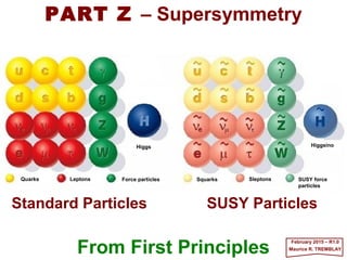
  • 1. From First Principles June 2017 – R4.0 Maurice R. TREMBLAY Standard Particles SUSY Particles PART IX – SUPERSYMMETRY Higgs Higgsino Quarks SquarksLeptons SleptonsForce particles SUSY force particles
  • 2. Supersymmetry is a symmetry that unites particles of integer and half-integer spin in common symmetry multiplets (e.g., a group of related subatomic particles) – it is a symmetry connecting bosons and fermions. It is a possible symmetry of nature in four space-time dimensions and it has the quality of uniqueness that physicists search for in fundamental physical theories. There is an infinite number of Lie groups that can be used to combine particles of the same spin in ordinary symmetry multiplets, but there are only eight kinds of supersymmetry in four space-time dimensions, of which only one, the simplest, could be directly relevant to observed particles. Unfortunately, there is still no direct evidence for supersymmetry, as no pair of particles related to supersymmetry transformations has yet been discovered. There is one significant piece of indirect evidence for supersymmetry: the high-energy unification of the SU(3)C⊗SU(2)L⊗U(1)Y gauge couplings works better with the extra particles called for by supersymmetry than without them. Or maybe the problem might still reside with the point particle concept*. Forward 2 2017 MRT As with my other work, nothing of this is new or even developed first hand and frankly it is a rearranged compilation of various quotes from various sources (c.f., References) that aims to display an abridged but yet concise and straightforward mathematical developmentof supersymmetry(and some higher-dimensional theories too) as I understand it and wish it to be presented to the layman or to the inquisitive person. As a matter of convention, I have included the setting h≡c≡1 in most of the equations and ancillary theoretical discussions and I use the summation convention that implies the summation over any repeated indices (typically subscript-superscript) in an equation. * A point particle is an idealization of particles heavily used in physics. Its defining feature is that it lacks spatial extension.
  • 3. Contents 2017 MRT PART IX – SUPERSYMMETRY Motivation Introduction to Supersymmetry The SUSY Algebra Realizations of the SUSY Algebra The Wess-Zumino Model Lagrangian with Mass and Interaction Terms The Superpotential Supersymmetric Gauge Theory Spontaneous Breaking of Supersymmetry F-type SUSY Breaking D-type SUSY Breaking The Scale of SUSY Breaking The SUSY Particle Spectrum Supersymmetric Grand Unification General Relativity The Principle of Equivalence General Coordinates “Supersymmetry […] introduces, apart from the three obvious dimensions plus time, new ‘quantum’ dimensions that cannot be measured by numbers; they are ‘quantum’ (or ‘fermionic’) dimensions, like the spin of the electron.” Edward Witten, The Quest for Supersymmetry talk at the Perimeter Institute. Local Lorentz Frames Local Lorentz Transformations General Coordinate Transformations Covariant Derivative The Einstein Lagrangian The Curvature Tensor The Inclusion of Matter The Newtonian Limit Local Supersymmetry A Pure SUGRA Lagrangian Coupling SUGRA to Matter and Gauge Fields Higher-dimensional Theories Compactification The Kaluza Model of Electromagnetism Non-Abelian Kaluza-Klein Theories Kaluza-Klein Models and the Real World N=1 SUGRA in Eleven Dimensions References
  • 4. The idea that there may be a symmetry called supersymmetry (SUSY) that interrelates bosons and fermions is rather attractive. In particular, SUSY might help to solve the hierarchy problem discussed in PART VIII – THE STANDARD MODEL: Hierarchy Problem. We saw there that the origin of this problem is the difficulty of including fundamental scalar Higgs fields in the theory. Scalars are the only fields that can have nonzero vacuum expectation values (and so give spontaneous symmetry breaking) without breaking the Lorentz invariance of a theory. On the other hand, the masses of such scalars are subject to quadratically divergent renormalization corrections of the like of ∆MH 2 ∝[g2/(2π)4]∫ Λ (1/k2)d4k ~(g2/8π2)Λ2 and there is no natural way to sustain a light Higgs of mass O(MW) together with a heavy Higgs of O(MX). There will be radiative corrections to the light Higgs mass of O(MX) that automatically destroy the hierarchy. Only by an unnatural fine tuning of parameters, order-by-order in perturbation theory, could we keep a light Higgs of mass O(MW). A natural solution would be the existence of a symmetry that requires that certain scalars must have zero mass. Chiral symmetry ensures zero fermion masses by forbidding mass terms like mψRψL. This appears unlikely to help with scalars because the scalar mass term, m2φφ*, always respects this symmetry. However, in a supersymmetric model each scalar mass must be equal to that of its fermion partner, which can be required to vanish by chiral symmetry. Moreover, the scalar mass, MH, is then no longer quadratically divergent because the boson and fermion loop corrections in ∆MH 2 above have opposite signs and cancel each other: Motivation 4 2017 MRT0~~ fermion 22 boson 222 H =ΛΛ∆ ggM _
  • 5. We begin by introducing the generators of SUSY transformations, Q, which turns fermions F into bosons B and vice versa: 5 2017 MRT Owing to the fermionic character of Q, any supersymmetric multiplet must contain numbers of bosons and fermions of the same mass. Nature, however, is manifestly not supersymmetric. The known bosons and fermions do not group themselves into such mass-degenerate pairs. (N.B., the vacuum state is labelled by |0〉 regardless). FBBF == QQ and Although experimental support for supersymmetry is still lacking, many people believe (e.g., the likes of Edward Witten!) that it is too beautiful to have been discarded by nature, and that it is only a matter of time before evidence of SUSY, albeit in some broken form, will be found. We need a finite Higgs mass of O(MW) to produce the obser- ved electroweak symmetry breaking, so we want to break SUSY gently so that ∆MH 2 above becomes: )( 2 F 2 B 22 H mmgM −∝∆ So if this last equation is to give ∆MH 2 < MH 2, supersymmetric partners of the ordinary particles must be found with masses <1 TeV.~ ~ In the subsequent chapters we will give an introduction of the main ingredients of supersymmetric theories. For further technical details of the general formalism of SUSY, we suggest the References and note that the definitive authoritative reference seems to be Supersymmetry and Supergravity, 2nd Ed., Wess and Bagger (1992). Introduction to Supersymmetry
  • 6. Now, to illustrate how supersymmetry works, we begin with the following example, which includes many of the most important features of SUSY theories. Consider a simple harmonic oscillator with both bosonic and fermionic degrees of freedom. 6 2017 MRT 0],[],[1],[],[ †††††† ===≡≡− − bbbbbbbbbbbb and while those of the fermion (i.e., f † and f ) satisfy the anticommutation relations: 0},{},{1},{],[ †††††† ===≡≡+ + ffffffffffff and Since f †f †|0〉=0, two fermions cannot occupy the same state (i.e., Pauli’s exclusion principle). In terms of these operators, the Hamiltonian takes the form: ],[ω½},{ω½ † F † B ffbbH += where ωB and ωF are the classical frequencies of the boson and fermion oscillators, respectively, and the allowed energies are: )(ω)½(ω)½(ω FBFFBB nnnnE +=+++= if ωB =ωF =ω. In this supersymmetry limit we have exact cancellation of the zero-point energies! So, nF=0,1 are the only allowed eigenvalues of the fermion number operator, f †f, and so all the energy levels are doubly degenerate, except for the ground state (i.e., nB =nF=0). The system thus contains equal numbers of bosonic and fermionic degrees of freedom! The creation and annihilation operators of the boson (i.e., b†≡bcT and b, respectively, with † the Hermitian conjugate symbol which means that one has to transpose T the matrix then change the imaginary elements c from i to −i) satisfy the commutation relations:
  • 7. This degeneracy indicates that there must exist some (super)symmetry of the Hamiltonian. In fact, it is easy to check that the (annihilation and creation) charge operators*: 7 2017 MRT bfQfbQ ††† 22 ω=ω= and commute with the Hamiltonian H=P0 (e.g., Pµ =[P0,Pi]): 0],[],[ † == HQHQ with √(2ω) being just a simple normalization factor (Exercise). The operators Q and Q† clearly have the effect of replacing a fermion by a boson, and vice versa, as in Q|F〉=|B〉 and Q|B〉=|F〉 above, and so they are supersymmetry generators. Furthermore, we find that: HQQ 2},{ † = and so the algebra of Q, Q†, and H closes if we include anticommunication as well. This anticommutator is the essence of SUSY. * We present a tabular representation of these operators to help in the association later on or to help in memorizing this fact. bfQfbQ ††† 22 ω=ω= Replacing a: fermion by a boson boson by a fermion Supersymmetric charge generators Operators: This is explained in words by: A fermion is destroyed, f, and a boson is created, b†. A boson is destroyed, b, and a fermion is created, f †. √(2ω) is a normalization factor.
  • 8. In a 1967 paper, Sidney Coleman and Jeffrey Mandula (S.C.’s former Grad student) adopted reasonable assumptions about the finiteness of the number of particle types below any given mass, the existence of scattering at almost all energies, and the analyticity of the S-matrix, and used them to show that the most general Lie algebra of symmetry operators that commute with the S-matrix, that take single-particle states into single-particle states, and that act on multiparticle states as the direct sum of their action on single-particle states consists of the generators Pµ and Mµν of the Poincaré group, plus ordinary internal symmetry generators Ta that act on one-particle states with matrices that are diagonal in and independent of both momentum and spin. 8 2017 MRT ],,[],,[],,[],,[ 321030201321123123 KKKMMMJJJMMM =≡=≡ KJ and So, Coleman and Mandula showed that, under very general assumptions, a Lie group that contains both Poincaré group P and an internal symmetry G must be just a direct pro- duct of P and G. The generators of the Poincaré group are the four-momentum Pµ=[H,P], which produces space-time translations, and the antisymmetric tensor Mµν , which generates space(J)-time(K) rotations: The SUSY Algebra where the angular momentum operator J≡Jk generates space rotations about the k-axis and K≡Kk generates Lorentz boosts along the k-axis. So if the generators of the Coleman-Mandula theorem requires that: 0],[],[ == aa TMTP µνµ This no-go theorem shows the impossibility of combining space-time and internal symmetries in any but a trivial way (or else commutators such as [.,.]=1 would exist).
  • 9. Yet, formulating supersymmetry escapes this ‘no-go’ theorem because, in addition to the generators Pµ, Mµν , Ta which satisfy commutation relations, it involves fermionic generators Q that satisfy anticommutation relations. If we call the generators with these properties even and odd, respectively, then the SUSY algebra has the general structure: 9 2017 MRT odd]odd,even[even}odd,odd{even]even,even[ === and, which is called a graded Lie algebra by mathematicians. Without further ado we now present the simplest form of SUSY algebra. We introduce four generators Qα (α =1,…,4),which form a four-componentMajorana spinor. Majorana spinors are the simplest possible type of spinor. They are self-conjugate (i.e., ψ c =ψ ): T QCQQ c == and hence have only half as many degrees of freedom as a Dirac spinor. (N.B., we use for Q the same convention as the adjoint [row] Dirac spinor, ψ =ψ †γ 0). Indeed, any Dirac spinor ψ =[ψ1 ψ2 ψ 3 ψ 4]T may be written: )( 2 1 21 ψψψ i+= where: are two independent Majorana spinors that satisfy ψ i =ψ i c. )( 2 )( 2 1 21 cc i ψψψψψψ −−=+= and __
  • 10. Since Qα is a spinor, it must satisfy: 10 2017 MRT βαβµνµνα QMQ )( 2 1 ],[ Σ= where the sum over β is implicit (i.e., summation convention for repeated indices). This relation expresses the fact that the Qα transform as a spinor under the rotations generated by Mµν (N.B., Σµν =½i(γ µγ ν −γ νγ µ )=½i[γ µ,γ ν ], when sandwiched between spinors, transforms as an antisymmetric tensor). The Jacobi identity of commutators: requires that Qα must be translationally invariant: 0]],,[[]],,[[]],,[[ =++ ανµµαννµα QPPPQPPPQ 0],[ =µα PQ It is the remaining (anti)commutation relation (c.f., [Q,Q†]=2H of the Motivation chapter): µαβ µ βα γ PQQ )(2},{ = where the sum over µ is implicit, which we shall derive later on from first principles, and closes the algebra, that has the most interesting consequences. Clearly this {Qα ,Qβ} anticommutator has to yield an even generator, which might be either Pµ or Mµν . But a term of the form Σµν Mµν (sum over µν) on the right-hand side would violate a generalized Jacobi identity involving Qα, Qβ, and Pµ and the algebra would not close. Indeed, if we go back to the ‘no-go’ theorem and allow for anticommutators as well as commutators, we find that the only allowed supersymmetries are those based on the graded Lie algebra defined by [Qα ,Mµν ], [Qα ,Pµ], and {Qα ,Qβ} above. _ _
  • 11. We choose Qα to be a Majorana spinor with four independent (real) parameters, but we could have used a Weyl spinor with two complex components equally well. In fact, we shall find it more convenient to work with a left-handed Weyl spinor χa with a=1,2, and the chiral representation of the Dirac matrices in which: 11 2017 MRT      − =      =      − = I I I I 0 0 0 0 0 0 50 γγ and, σσσσ σσσσ γγγγ The charge-conjugation matrix, C, defined by the final equation, satisfies the require- ment: Realizations of the SUSY Algebra       − =      +      == *0 * 0 2 0 Q QQQ σ γ i CQQ c T In this chiral representation we find: c RLLL C ψψψγψψ +=+= * 0 T       − = 0 0 2 2 0 σ σ γ i i C T and: Using the two-component Weyl spinor Qa, we can construct a Majorana spinor Qα as in: T µµ γγ −=− CC 1
  • 12. We then look for possible SUSY representations that contain massless particles. These should be the relevant multiplets, since the particles we observe are thought to acquire their masses only as a result of spontaneous symmetry breaking. The procedure we employ is to evaluate the anticommutator {Qα ,Qβ} of the The SUSY Algebra chapter for a massless particle moving along the z-axis with Pµ =[E,0,0,E]. On substituting Q=Qc = [Q −iσ2 Q*]T above into {Qα ,Qβ}, we find: 12 2017 MRT E4},{0},{0},{ † 22 † 11 † 21 === QQQQQQ and, with a=1,2, giving: abba E )1(2},{ 3 † σ−=QQ We see that Q2 † and Q2 act as creation and annihilation operators, respectively, just like f † and f in { f , f †}=1 and { f , f }={ f † , f †}= 0 of the Motivation chapter. _ _
  • 13. Now a massless particle of spin s can only have helicities λ=±s, so, starting from the left-handed state |s,λ=−s〉, which is annihilated by Q2, only one new state can be formed (i.e., Q2 †|s,−s〉). This describes a particle of spin s+½ and helicity −(s+½), and by virtue of [Qα ,Pµ]=0 of the The SUSY Algebra chapter, it is also massless. Then, acting again with Q1 † or with Q2 † gives states of zero norm by virtue of {Q1,Q2 †}=0, {Q1,Q1 †}=0, and also {Q2 ,Q2 †}=4E above and note that Q2 †Q2 †=0 (which follows from the fermionic nature of Q2). So the resulting massless irreducible representation consists of just two states. Hence, the possible supersymmetric multiplets {|s,λ〉} of interest to us are: 13 2017 MRT                 ½,½ 2,1 0,0 ½,½ gauginosfermion bosongaugefermion multipletgauge)(orVectormultipletChiral To maintain CPT invariance we must add the antiparticle states that have opposite helicity, thus giving a total of four states, |s+½, ±(s+½)〉, |s, ±s〉, in each multiplet. All the particles in such multiplets must carry the same gauge quantum numbers. For this reason, the known fermions (i.e., the quarks and leptons) must be partnered by spin-0 particles (called sfermions), not spin-1 bosons. This is because the only spin-1 bosons allowed in a renormalizable theory are the gauge bosons and they have to belong to the adjoint representation of the gauge group, but the quarks and leptons do not. Instead, the gauge bosons are partnered by new spin-½ gauginos(spin-3/2 being ruled out by the requirement of renormalizability).
  • 14. There is of course no experimental evidence for the existence of such spin-0 sfermions or spin-½ gauginos. The need to introduce new supersymmetric partners, rather than interrelate the known bosons and fermions, is undoubtedly a major setback for SUSY. 14 2017 MRT For completeness, we briefly consider also supermultiplets of particles with nonzero mass M. In this case, in the particle’s rest frame, Pµ=[M,0,0,M], so the anticommutator {Qα ,Qβ}=2(γ µ)αβ Pµ of the The SUSY Algebra chapter becomes: abba Mδ2},{ † =QQ We see that Qa †/√(2M) and Qa/√(2M) act as creation and annihilation operators, respectively, for both a=1 and 2. Starting from a spin state |s, s3〉, which is annihilated by the Qa, we can reach three other states by the action of Q1 †, Q2 † and Q1 †Q2 † =−Q2 †Q1 †. For example, from the spin states |½, ±½〉 we obtain: and hence generate a SUSY multiplet consisting of one spin-0, one spin-1 and two spin-½ particles, all of mass M. |½, ½〉 |½, −½〉 |1, 1〉 |1, 0〉, |0, 0〉 |½, ½〉 |½, −½〉 |1, −1〉 χ1 † χ2 † χ1 † χ2 † χ2 † χ1 † χ2 † χ1 † _
  • 15. In summary, supersymmetry is a symmetry that relates bosons to fermion (i.e., schematically a SUSY generator Q acts as Q(fermion)=boson and Q(boson)=fermion) and so requires an equal number of fermionic and bosonic degrees of freedom. 15 2017 MRT ∫ ∂−Φ∂Φ−∂= )*(4 ψσψ µ µ µ µ ixdS The simplest 4D system invariant under SUSY is a free theory with Weyl fermions ψα and a complex scalar Φ, whose action is: Now, if we consider the convention of a metric with signature [−,+,+,+] and the Weyl spinor notation of Wess and Bagger, we have 2-component spinors with undotted and dotted indices ψα ,ψ α , transforming in representation (½,0) and (0,½) of the Lorentz group. A Dirac spinor contains two Weyl spinors, ΨD=(ψα ,χα ), and a Dirac mass term reads ψ αχα +ψα χα. Some useful identities are ψχ =ψ αχα =−ψα χα =χαψα =χψ. One also defines [σ µ αα ]=[−I,σσσσ] and [σ µ αα ]=[−I,−σσσσ], where I is the 2×2 identity matrix and σσσσ the 2×2 Pauli spin matrices. ⋅⋅⋅⋅ ⋅⋅⋅⋅ ⋅⋅⋅⋅ ⋅⋅⋅⋅ ⋅⋅⋅⋅ ⋅⋅⋅⋅ This system has a current which is conserved on-shell (i.e., upon use of the equations of motion). This so-called supercurrent is: 0)*( =∂Φ∂= µ αµα µν ν µ α ψσσ JJ with which implies the conservation of the (super)charges: ∫∫ == 0303 αααα && JxdQJxdQ and _ _ _ _
  • 16. These charge generators have the unusual properties of being fermionic and transforming as Weyl spinors under the Lorentz group – rather than scalars, as more familiar symmetry generators. Also their algebra is generated by anticommutation relations, rather than by commutators. Since both Q and Q are conserved, their anticommutator should be a bosonic conserved quantity. The only candidate in the space-time momentum Pµ, necessarily contracted with σ µ to have the right spinorial structure. Indeed explicit computation leads to the (super)algebra: 16 2017 MRT µ µ αααα σ PQQ && 2},{ = with other (anti)commutators vanishing: 0],[],[},{},{ ==== µαµαβαβα PQPQQQQQ &&& Remarkably, Qα and Qα are not generators of an internal symmetry, rather they intertwine with the Poincaré algebra. You can compare this to the form obtained earlier: ⋅⋅⋅⋅ µαβ µ βα γ PQQ )(2},{ = with: These are similar but do not highlight the spinorial nature of the Wess and Bagger notation (as it is widely used in the community). Since the content here is really to show the features of supersymmetry I revert back to the original Majorana notation.       =      − = 0 0 0 0 0 I I γand σσσσ σσσσ γγγγ _ _
  • 17. We are now ready to consider the construction of supersymmetric field theories such as the Wess-Zumino Model [Supergauge transformations in four dimensions, Nuclear Physics B 70 (1): 39–50 (1974). Look up this title here: http://booksc.org] of the massless spin-0–spin-½ multiplet, which in some way, is an alternative introduction to SUSY. Indeed, probably the most intuitive way of introducing SUSY is to explore, through this simple example, possible Fermi-Bose symmetries of the Lagrangian. It could therefore equally well have been the starting point for our discussion of SUSY. 17 2017 MRT ψγψ µ µµ µ µ µ ∂+∂∂+∂∂= iBBAA 2 1 ))(( 2 1 ))(( 2 1 L The simplest multiplet in which to search for SUSY consists of a two-component Weyl spinor (or equivalently a four-component Majorana spinor) together with two real scalar fields. To be specific, we take a massless Majorana spinor field,ψ, massless scalar field, A, and massless pseudoscalar field, B. The kinetic energy is: The Wess-Zumino Model with ψ =ψ †γ 0, as usual. The unfamiliar factor of ½ in the fermion term arises because ψ is a Majorana spinor; a Dirac spinor ψ =[ψ1 ψ2 ψ3 ψ4]T is a linear combination of two Majorana spinors (c.f., ψ =(1/√2)(ψ1+iψ2)). The following bilinear identities are particularly useful when exploring SUSY. For any two Majorana spinors ψ1, ψ2 we have: 1221 ψψηψψ Γ=Γ where η=(1,2,−1,1,−1) for Γ={1,γ5 ,γµ ,γµγ5 ,Σµν}. These relations follow directly from when we recall that Majorana spinors are self-conjugate, ψi c=ψi. _
  • 18. To discover the Fermi-Bose symmetries of L, we make the following infinitesimal transformations: 18 2017 MRT ψδψψψδδ +=′→+=′→+=′→ and, BBBBAAAA where: where ε is a constant infinitesimal Majorana spinor that anticommutes with ψ and commutes with A and B. So, overall, these transformations then look like: εγγψδψγεδψεδ µ µ )( 55 BiAiiBA +∂−=== and, _ _ These transformations are Lorentz-covariant but otherwise δ A and δ B are just fairly obvious first guesses. ψγε ψε 5iBB AA +=′ +=′ and: εγγψψ µ µ )( 5BiAi +∂−=′ The possibility of constructing two independent invariant quantities εψ and εγ5ψ and ψ have mass dimensions 1 and 3/2, respectively, ε must have dimension −½. Hence, the derivative in δψ is therefore required to match these dimensions. We have also assumed that the transformations have to be linear in the fields.
  • 19. Under the transformations δ A=εψ, δ B=iεγ5ψ, and δψ =−iγ µ∂µ(A+iγ5B)ε above the change in L can be written in the form: 19 2017 MRT where we have used the identities:       +∂/∂=             +∂−+∂∂= +∂∂+∂+∂−∂∂+∂∂= ∂+∂+∂∂+∂∂= ∂+∂+∂∂+∂∂+∂∂+∂∂= ∂+∂+∂+∂∂+∂∂+∂∂+∂∂= ∂+∂∂+∂∂= ψγγε ψγγγγε εγγγψψγγγεψγεψε ψδγψψγψδδδ ψδγψψγψδδδδδ ψδγψψγδψψγψδδδδδ ψγψδδδδ µ µ ν µνµ µ ν ν µ µ µν µν µ µ µ µ µ µ µ µ µ µ µ µ µ µ µ µµ µ µ µ µ µ µ µ µ µ µ µ µ µµ µ µ µ µ µ µ µ µ µµ µ µ µ )]([ 2 1 )( 2 1 )( ])([ 2 1 )( 2 1 )( 2 1 )( 2 1 )()( )]()[( 2 1 )]()([ 2 1 )]()([ 2 1 )]()()([ 2 1 )]()([ 2 1 )]()([ 2 1 )( 2 1 )( 2 1 )( 2 1 5 55 555 BiA BiABiA BiABiABiA iiBBAA iBBBBAAAA iBBBBAAAA iBBAAL εγψψγεεψψε 55 == and of ψ1Γψ2 =ηψ2Γψ1 above where η=(1,2,−1,1,−1) for Γ={1,γ5,γµ,γµγ5,Σµν}. Since δ L is a total derivative, it integrates to zero when we form the action. Hence, the action is invariant under the combined global supersymmetric transformations δ A=εψ, δ B= iεγ5ψ, and δψ =−iγ µ∂µ(A+iγ5B)ε that mix the fermion and boson fields. As usual, global is used to indicate that ε is independent of space-time (also termed rigid). __ __ _ _
  • 20. We have remarked that the δψ transformation (i.e., −iγ µ∂µ(A+iγ5B)ε) contains a derivative. It thus relates the Fermi-Bose symmetry to the Poincaré group. In particular, the appearance of the time derivative (i.e., ∂µ≡∂/∂xµ =[∂/∂t,∇∇∇∇]) gives an absolute significance to the total energy, which is normally absent in theories that do not involve gravity. This could be relevant to the value of the cosmological constant Λ. 20 2017 MRT When we extend the global supersymmetry of this chapter to local supersymmetry, the presence of derivatives in the algebra will imply that derivatives at different points of space-time are related. This has the implications for the metric of space-time and will take us into the domain of general relativity. We shall find that when we come to construct Lagrangians that are supersymmetric under local supersymmetry transformations we shall be forced to introduce a spin-2 particle that can be identified with the graviton. Thus, gravity naturally and automatically becomes unified with the other forces of physics, which is why local supersymmetry is called supergravity (SUGRA). This enhances the interest of super theories. It is quite amazing that spin-2 particles (but none higher!) are naturally introduced by these limited requirements of Fermion-Boson statistics, anticommutator-commutator graded Lie algebras, and space-time locality. These very convincing arguments are used to explain the rationale suggesting that nature was supersymmetric in its origin and that what we see today is just the condensation of particle states (because the universe is so cold!) and that spontaneous symmetry breaking occurred often in the past. Of course, the mechanisms inherently used by particle interactions and the continuous and per- sisting issue of finding a true universal vacuum occupies most of physics even today!
  • 21. Returning our attention again to the global transformations δ A=εψ, δ B=iεγ5ψ, and δψ =−iγ µ∂µ(A+iγ5B)ε above, we recall that the commutator of two successive transformations of a symmetry group must itself be a symmetry transformation. In this way we identified the algebra of the generators of the group. To obtain the corresponding result for supersymmetry, we must therefore consider two successive SUSY transformations like δ A, δ B, and δψ. For example, if for the scalar field A we make a transformation δ A=εψ associated with parameter ε1, followed by another with parameter ε2, then we obtain from δψ =−iγ µ∂µ(A+iγ5B)ε: 21 2017 MRT 2511212 )()()( εγγεψεδδδ µ µ BiAA +∂−== Hence, the commutator: AP AiAi BiAiBiAiAA µ µ µ µ µ µ µ µ µ µ εγε εγεεγε εγγεεγγεδδδδδδ 21 2121 152251122112 2 )(22 )()(],[)( −= ∂−=∂−= +∂++∂−==− since the terms involving B cancel when we use identities for Majorana spinors (i.e., the ψ1Γψ2 =ηψ2Γψ1 relation above where η=(1,2,−1,1,−1) for Γ={1,γ5,γµ,γµγ5,Σµν }) and, of course, i∂µ=Pµ. _ _ _ __
  • 22. Now the generator of SUSY transformations Qα is a four-component Majorana spinor, which we define by the requirement that (c.f., φ →exp(iα)φ ≈(1+iα)φ ≡φ +δφ and φ*→ exp(−iα)φ*≈(1−iα)φ*≡φ* +δφ*): 22 2017 MRT AQA εδ = To make this consistent with [δ2 ,δ1]A=−2ε1γ µε2 Pµ A above, we form the commutator: AQQ AQQQQ AQQ AQQA },{ )( ],[ ],[],[ 21 2112 12 1212 βαβα ββααααββ εε εεεε εε εεδδ = −= = = using εψ =ψε and ε γ 5ψ =ψγ 5ε. Writing [δ2 ,δ1]A= −2ε1γ µε2 Pµ A in component form and equating it with the last commutator, [δ2 ,δ1]A=−ε1α ε2β {Qα ,Qβ}A, reveals the basic SUSY requirement: µαβ µ βα γ PQQ )(2},{ = which is indeed part of SUSY algebra {Qα ,Qβ} obtained earlier in the Motivation chapter. _ _ _ _ _ _ _ _ _
  • 23. Without going into detail, the algebra closes when acting on the spinor field ψ : 23 22 aux 2 1 2 1 GFL += However, there is a problem with [δ2 ,δ1]ψ =−2iε1γ µε2 ∂µψ +iε1γ νε2 γν ∂ψ above because it gives the required closure only when ψ satisfies the free Dirac equation, but not for interacting fermions that are off the mass shell. The reason is that for off-mass- shell particles the number of fermions and boson degrees of freedom no longer match up. A and B still have two bosonic degrees of freedom, whereas the Majorana spinor ψ has four. We can restore the symmetry by adding two extra bosonic fields, F and G (called auxiliary fields because it appears without derivatives in the action hence no dynamics associated to them), whose free Lagrangian takes the form: 2017 MRT ψγεγεψεγε εψγεγεψεεψγεγεψε εγδγεγδγψδδ ν ν µ µ µ µ µ µ ∂/+∂−= +∂/−+∂/−= +∂−+∂−= 2121 251521152512 25115212 2 )()( )()(],[ ii iiiiii BiAiBiAi If we use the field equation ∂ψ =0 for a free massless fermion, the last term vanishes identically and [δ2 ,δ1]ψ above has the same form [δ2 ,δ1]ψ =−2ε1γ µε2 Pµψ (same as above for the field A) and hence we again obtain {Qα ,Qβ}ψ =−2(γ µ)αβ Pµ as above. This gives the field equations F=G=0, so these new fields have no on-mass-shell states. _ _ _
  • 24. From Laux =½ F 2 +½ G2 above they clearly must have mass dimension 2, so on dimensional grounds their SUSY transformations can only take the forms: 24 ψγγεδψγεδ µ µ µ µ ∂=∂−= 5 GiF and and δψ =−iγ µ∂µ(A+iγ5B)ε above then becomes: 2017 MRT εγεγγψδ µ µ )()( 55 GF iBiAi +++∂−= The mass dimensions prevent F and G from occurring in: ψγεδψεδ 5iBA == and Under these modified SUSY transformations (i.e., the unchanged δ A=εψ, δ B=iεγ5ψ, and the corrected δψ =−iγ µ∂µ(A+iγ5B)ε +(F+iγ5G)ε above), we can show that the unwanted term in [δ2 ,δ1]ψ = −2iε1γ µε2 ∂µψ +iε1γ νε2 γν ∂ψ above cancels and, moreover, that: FF µ µ εγεδδ ∂−= 2112 2],[ i and similarly for G, as required by {Qα ,Qβ}ψ =−2(γ µ)αβ Pµ above. In this way, we have obtained the spin-0–spin-½ realization of SUSY originally found by Wess and Zumino in 1974 (c.f., http://booksc.org/book/16430412.) _ _ __ _
  • 25. We have found that the free Lagrangian: 25 that describes the multiplet (A,B,ψ, F, G), is invariant (up to a total derivative) under the SUSY transformations: 2017 MRT Lagrangian with Mass and Interaction Terms 22 o 2 1 2 1 2 1 2 1 2 1 GFL ++∂/+∂∂+∂∂= ψψµ µ µ µ iBBAA       −+= ψψ 2 1 BAmm GFL and a cubic interaction term: ])(2[ 2 5 22 nInteractio ψγψ BiABABA g −−+−= GFFL Higher-order terms must be excluded because they are nonrenormalizable. However, SUSY invariance is still preserved if the Lagrangian is extended to include a quadratic mass term of the form: ψγεδ ψεδ 5iB A = = and εγεγγψδ µ µ )()( 55 GF iBiAi +++∂−=
  • 26. When we use the classical equation of motion: 26 These equations of motion are purely algebraic and so the dynamics is unchanged if we use them to eliminate the auxiliary fields F and G from the Lagrangian. We then obtain: 2017 MRT 0= ∂ ∂ = ∂ ∂ G L F L for the complete Lagrangian, L = Lo + Lm + LInteraction, we find: 0)( 2 22 =+++ BA g AmF ψγψ ψψψψµ µ µ µ )( 2 )( 4 1 )( 2 )( 2 1 2 1 22 1 2 1 5222222222 BiA g BAgBAAm g BAm m i BBAA −−+−+−+− −∂/+∂∂+∂∂=L Several features of this Lagrangian, which are characteristic of supersymmetric theories, are worth noting. The masses of the scales and the fermion are all equal. There are cubic and quartic couplings between the scalar fields, and also a Yukawa-type interaction between the fermion ψ and the scalars A and B, yet in total there are only two free parameters: m and g. This interaction between boson and fermion masses and couplings is the essence of SUSY. 02 =++ BAgBmG and:
  • 27. The model can also be shown to have some remarkable renormalization properties in that, despite the presence of the scalar fields, there is no renormalization of the mass and coupling constant (although wave function renormalization is still necessary). The divergences arising from boson loops are cancelled by those of fermion loops which have the opposite sign. This is just the type of cancellation we need to stabilize the gauge hierarchy. 27 2017 MRT These powerful nonrenormalization theorems make SUSY particularly compelling. However, when we break SUSY, as we must given the absence of fermion-boson mass degeneracy in nature, we have to be careful to preserve the relation between the couplings of particles of different spin embodied in our L above.
  • 28. To see how these results generalize with higher symmetries, it is convenient to work entirely with left-handed fermion fields (c.f., PART VIII – THE STANDARD MODEL: Possible Choices of the Grand Unified Group chapter). A Majorana spinor ψ can be formed entirely from a left-handed Weyl spinor: 28 T LL Cψψψ += where C is the charge-conjugation matrix and that the mass term is: 2017 MRT The Superpotential h.c.h.c. +=+= LLL c R Cmmm ψψψψψψ T using ψL c ≡ψL c †γ0 =ψR*†γ0 T†C†γ0= −ψR T C−1(=ψR TC) and +h.c. means add the Hermitian conjugate. For simplicity we have set −C−1 =C, which is valid in all the familiar representations of the Dirac matrices. _
  • 29. We can rewrite the SUSY Lagrangian of the Lagrangian with Mass and Interaction Terms chapter using just a single left-handed field ψL, and complex field φ and F for its scalar partners: 29 2 * φφ gmF −−= Then, using the equation of motion ∂ L/∂F=0, which gives: 2017 MRT )( 2 1 )( 2 1 GF iFBiA −≡+≡ andφ From L = Lo + Lm + LInteraction, we obtain: h.c.)( h.c. 2 1 ** 2 +−+ +      −+ +∂/+∂∂= LL LL LL CFg CFm FFi ψψφφ ψψφ ψψφφ µ µ T T L we can eliminate the auxiliary field F* and so the Lagrangian becomes:       ++−+−∂/+∂∂= h.c 2 1 * 2 2 LLLLLL CgCmgmi ψψφψψφφψψφφ µ µ TT L (c.f., Lagrangian of the Lagrangian with Mass and Interaction Terms chapter).
  • 30. It is useful to re-expressthefirst Lagrangianof this chapter (i.e., L = Lo + Lm + LInteraction) in terms of an analytic function W(φ), known as the superpotential: 30 where LKE denotes the sum of the kinetic energy terms of the φ and ψL fields. (N.B., W, which is of dimension 3, depends on φ and not on φ*). Upon using ∂ L/∂F=∂ L/∂F*=0 to eliminate the auxiliary fields, we find: 2017 MRT         + ∂ ∂ − ∂ ∂ + ∂ ∂ ++= h.c. 2 1 * * ** 2 2 KE LL C WW F W FFF ψψ φφφ T LL         + ∂ ∂ − ∂ ∂ −= h.c. 2 1 2 22 KE LL C WW ψψ φφ T LL For a renormalizable theory W can be, at most, a cubic function of φ, since otherwise the Lagrangian would contain couplings with dimension less than 0. Substituting: 32 3 1 2 1 φφ gmW += into our last Lagrangian L = LKE +|∂W/∂φ|2−½[(∂2W/∂φ2)ψL T CψL +h.c.] above imme- diately reproduces the L =∂µφ∂µφ*+iψL ∂ψL −|mφ +gφ2|2 −(½mψL T CψL +gφψL T CψL +h.c.) Lagrangian derived earlier. The superpotential is the only free function in the SUSY Lagrangian and determines both the potential of the scalar fields, and the masses and couplings of the fermions and bosons. _
  • 31. In general there may be several chiral multiplets to consider. For example, if ψ i belongs to a representation of an SU(N) symmetry group, we will have the supermultiplets: 31 ),( i L i ψφ where in the fundamental representation i=1,2,…,N. From the derived Lagrangian L = LKE +|∂W/∂φ|2 −½[(∂2W/∂φ2)ψL T CψL +h.c.] above we readily obtain a Lagrangian that is under the additional symmetry and incorporates the new supermultiplets. It is: 2017 MRT         + ∂∂ ∂ − ∂ ∂ −∂/+∂= ∑∑∑∑ h.c. 2 1 22 2 Chiral ji j L i Lji i i i i L i L i i C WW i ψψ φφφ ψψφµ T L and the most general form of the superpotential W is: kji kji ji ji i i gmW φφφφφφλ 3 1 2 1 ++= where the coefficients m and g are completely symmetric under interchange of indices. Since W must be invariant under SU(N) symmetry transformations the term linear in the fields can only occur if a gauge-singlet field exists.
  • 32. A combination of SUSY with gauge theory is clearly necessary if these ideas are to make any contact with the real world. In addition to the chiral multiplet (φi,ψL i) (i=1,2,…, N) we must include the gauge supermultiplets: 32 ),( aa A χµ with a=1,2,…,N2 −1 and where Aµ a are the spin-1 gauge bosons of the gauge group G (taken to be SU(N)) and χa are their Majorana fermion superpartners (the so-called gauginos). These boson-fermion pairs, which in the absence of symmetry breaking are assumed to be massless, belong to the adjoint representation of the gauge group. Our task is to find a SUSY- and gauge-invariant Lagrangian containing all these chiral and gauge supermultiplets. 2017 MRT Supersymmetric Gauge Theory The gauge multiplets are described by the Lagrangian (N.B., a,b,c=1,…, 8): 2 Gauge )( 2 1 )( 2 1 4 1 a a a a a DDiFF +/+−= χχµν µνL where the gauge field-strength tensor is (c.f., PART VIII – THE STANDARD MODEL: Quantum Chromodynamics (QCD) chapter – Ga µν=∂µGa ν −∂ν Ga µ −gs fabcGb µGc ν ): νµµννµµν cbabcaaa AAfgAAF Gauge−∂−∂= Dµ is the covariant derivative satisfying (c.f., op cit: Spontaneous Symmetry Breaking in SU(5) chapter – (DµΦ)K= ∂µΦK +ig[(TI Aµ I)KJ ΦJ] – N.B., I,J,K=1,…,24): caabcaa AfgD χχχ µµµ Gauge)( −∂= and Da is an auxiliary field (similar to Fi of the chiral multiplet).
  • 33. Actually, for this pure gauge Lagrangian the equation of motion, ∂ LGauge /∂Da =0, implies Da =0; however, it will become nonzero when the chiral fields are coupled in. The notation will be familiar: gGauge and fabc are the coupling and structure constants of the gauge group, and in the equation for (Dµχ)a above, the matrices Tb representing the generators in the adjoint representation have been replaced by (Tb)ac =i fabc. It is straightforward to show that LGauge is invariant, and that the algebra closes, under SUSY transformations: 33 εγχδ χγγεδ µν µν µµ 5 5 2 1 aa aa F A Σ−= −= where ε is a constant infinitesimal Majorana spinor. This transformation is analogous to δ A=εψ, δ B=iεγ5ψ, and δψ =−iγ µ∂µ(A+iγ5B)ε (c.f., Wess-Zumino Model chapter) for chiral multiplets. 2017 MRT _ _ aa DiD )( χεδ /−= and
  • 34. To include the chiral fields (φi,ψL i), we add LChiral of the The Superpotential chapter but substitute derivative Dµ for ∂µ in the kinetic energy terms: 34 aa ATgiD µµµµ Gauge+∂=→∂ where Ta are the matrices representing the generators of the gauge group in the representation to which (φi,ψi) belong. To ensure the supersymmetry of the combined chiral + gauge Lagrangian, we must include two further terms, and write: 2017 MRT ]h.c.)(2[)( * Gauge * GaugeGaugeChiral ++−+= jLji aa i a jji a i PTgDTg ψχφφφLLL where PL ≡½(1−γ 5), and also replace ∂µ in δ A=εψ, δ B=iεγ5ψ, and δψ =−iγ µ∂µ(A+iγ5B)ε +(F+iγ5G)ε of the Wess-Zumino Model chapter by Dµ. Model building begins with this SUSY Lagrangian. Using ∂ L /∂Da =0 to eliminate the auxiliary field gives: jji a i a TgD φφ )(* Gauge= The terms in the Lagrangian that contribute to the potential for the scalar fields are evident by inspection of L = LKE +|∂W/∂φ|2 −½[(∂2W/∂φ2)ψL T CψL +h.c.] and LGauge = −¼Fµν aFµν a+½iχa(Dχ)a +½(Da)2. They are: ∑ ∑∑         + ∂ ∂ =+= a ji jji a i i i ai Tg W DFV 2 * Gauge 2 22 )( 2 1 2 1 *),( φφ φ φφ which are known as the F and D terms, respectively. This potential will play a central role in the spontaneous breaking of SUSY and the gauge symmetry. _ _ _
  • 35. The particles observed in nature show no sign whatsoever of a degeneracy between fermions and bosons. Even the photon and neutrino, which appear to be degenerate in mass, cannot be SUSY partners. Hence, supersymmetry, if it is to be relevant to nature, must be broken. 35 0],[ ≠HQα The breaking could be either explicit or spontaneous: 2017 MRT Spontaneous Breaking of Supersymmetry and so the violation would have to be small enough to preserve the good features of SUSY and yet large enough to push the supersymmetric partners out of reach of current experiments. However, we would inevitably lose the nice nonrenormalization theorems and, even worse, any attempt to embrace gravity via local SUSY would be prohibited. 2. So instead we prefer to consider the spontaneous breaking of SUSY, not least because this has proved so successful previously for breaking gauge symmetries. Hence, we assume that the Lagrangian is supersymmetric but that the vacuum state is not: 0],[ =HQα 1. Explicit breaking would be quite ad hoc. The SUSY generators would no longer commute with the Hamiltonian: and: 00 ≠αQ
  • 36. A new feature arises here, however. The Higgs mechanism of spontaneous symmetry breaking is not available in SUSY because, if we were to introduce a spin-0 field with negative mass-squared, its fermionic superpartner would have an imaginary mass. Also, using the anticommutator {Qα ,Qβ}=2(γ µ)αβ Pµ of the The SUSY Algebra chapter: 36 ∑∑ += α α α α 2 †2 00008 QQH we can directly establish a general and important theorem. If we multiply this last commutator by γ 0 αβ and sum over β and α, we obtain: 2017 MRT µαβ µ βδδα γγ PQQ 2},{ 0† = HPQQ 88},{ 0 † ==∑α αα and hence: It follows immediately that: 1. the vacuum energy must be greater that or equal to zero; 2. if the vacuum is supersymmetric (i.e., if Qα |0〉=Q† α |0〉=0 for all α), the vacuum energy is zero; and 3. conversely, if SUSY is spontaneously broken (i.e., if Qα |0〉≠0), then the vacuum energy is positive. _
  • 37. These results have a disappointing consequence. Conclusion (1) gives an absolute meaning to the zero of energy, a fact that is was hoped to use to explain why the vacuum energy of the universe (represented by the cosmological constant Λ), is zero or very close to zero. But now from (3) we see that broken SUSY implies a positive vacuum energy. So small we find Λ=0 when we come to couple SUSY to gravity? Fortunately, the situation can be redeemed because the coupling to gravity introduces non-positive- definite terms in the scalar potential and a delicate cancellation can occur that may leave Λ≅0; but the puzzle of why Λ is zero (i.e., 10−122!) to such high precision is still not solved! [c.f., S. Weinberg, Rev. Mod. Phys., 61, 1 (1989)]. 37 Leaving this aside we can see from (3) that SUSY breaking is rather special because it requires the ground-state energy to be positive. In the classical approximation, the energy of the ground state is given by the minimum of the scalar potential V(φ,φ*)=|Fi|2 + ½Dα 2 of the Supersymmetric Gauge Theory chapter: 2017 MRT ∑ ++ ∂ ∂ = αβ β α β δηφφ φ 2 1 * Gauge 2 ])([ 2 1 jjii i Tg W V with: kjikjijijiii gmW φφφφφφλ 2 1 2 1 ++= The sum overβ has been included to allow for the possibility of different gauge groups with different couplings, and the constanttermη can only occur if β labels a U(1) factor.
  • 38. It is evidently hard to break SUSY. The minimum V =0 will occur when φi =0 for all i (and so SUSY will be unbroken) unless one of the following conditions applies: 38 ψδφψδψφδ ∂/+∂/ ~~~ FF and, 1. λi ≠0, that is, there exists a gauge-singlet field φi, so the superpotential W can contain a linear term yet still be gauge invariant (F-type breaking); 2. η ≠0, so the gauge group contains an Abelian U(1) factor (D-type breaking). This is a necessary but not a sufficient requirement. This mechanism cannot occur in GUTs because they are based on simple gauge groups that do not have U(1) factors. 2017 MRT There is an alternative way of seeing that the spontaneous symmetry breaking of SUSY can only be accomplished by 〈F〉≠0 and/or 〈D〉≠0. If we look back at the multiplet (φ,ψ,F), which takes the form: and from δ Aµ a =−ε γ µγ 5χa, δ χa =−½ΣµνFµν aγ5ε +Daε, and δDa =−iε(Dχ)a of the Supersymmetric Gauge Theory chapter for the gauge multiplet (Aµ ,χ,D), in which: χδχδχγδ µν µν µµ ∂/+Σ ~~~ DDFA and, and note that the vacuum expectation values of the spinor and tensor fields and ∂µφ must be zero to preserve the Lorentz invariance of the vacuum, then it is only possible to break the symmetry through nonzero vacuum expectation values of the auxiliary fields F and D. _ _
  • 39. The spontaneous breaking of SUSY requires: 39 00 ≠αQ and Qα |0〉 is necessarily a fermionic state, which we denote by |ψGauge〉. Since the Qα commute with H, the state |ψGauge〉 must be degenerate with the vacuum. It must therefore describe a massless fermion (with zero momentum). The situation is thus exactly analogous to the spontaneous breaking of an ordinary global symmetry in which massless Goldstone bosons are created out of the vacuum (c.f., PART VIII – THE STANDARD MODEL: Spontaneous Symmetry Breaking (SSB) chapter). Here the spontaneous breaking of global SUSY implies the existence of a massless fermion, which is called the Goldstino. 2017 MRT We next consider examples of these types of symmetry breaking, F-type and D-type introduced in (1) and (2) above.
  • 40. We now consider the O’Raifeartaigh (pronounced O’RAFFerty) Model which is a simple example of SUSY breaking arising from the presence of a linear term in the superpotential W: 40 2 BAgCBmAW ++−= λ which contains three complex scalar fields A, B, and C. In this example the scalar potential V =|∂W/∂φi|2 +½Σβα[gβ φi*(T α β)ijφj +ηδβ1]2 (with W=λiφi +½φi φj +⅓gijkφi φj φk ) of the Spontaneous Breaking of Supersymmetry chapter becomes: 2017 MRT F-type SUSY Breaking 2222 222 22 BmBAgCmBAgCmBg C W B W A W V ++++++−= ∂ ∂ + ∂ ∂ + ∂ ∂ = λ and see that V =0 is excluded because the last term is only zero if B =0 , but then the first term is positive-definite. We conclude the V >0 and that SUSY is broken. Provided m2 > 2gλ the potential V has a minimum when B =C =0, independent of the value of A. For simplicity, we set A =0 at the minimum.
  • 41. As usual (c.f., ∂V/∂φi|φ =v =0 and ∂2V/∂φi∂φj|φ =v =Mij 2 >0 of the PART VIII – THE STANDARD MODEL: Spontaneous Symmetry Breaking (SSB) chapter) the scalar masses are determined by evaluating: 41 at the minimum. The only nonzero elements are: 2017 MRT . 2 c&, BA V VAB ∂∂ ∂ ≡ 2 **** 2 mVVgVV CCBBBBBB ==−== andλ We see that the scalar field A remains massless and that the field C has mass m. SUSY breaking splits the mass of the complex B field because: 2 2 22 1 22 *** 2 )2()2(**2 BgmBgmBVBBVBV BBBBBB λλ ++−=++ where B=(1/√2)(B1+iB2), and so the real scalar fields B1 and B2 have [mass]2 =m2 m2gλ, respectively.
  • 42. The fermion masses are obtained by evaluating ∂2W/∂A∂B, &c., at the minimum (c.f., LChiral of the The Superpotential chapter). From W=−λ A+mBC+ gAB2 above we find that the only nonzero terms is: 42 and so the fermion mass matrix takes the form: 2017 MRT m CB W = ∂∂ ∂2           = 00 00 000 F m mM in the basis of the Majorana spinors ψA , ψB , ψC. The massless Goldstino state ψA is evident, and the ‘off-diagonal’ structure signals that the two Majorana spinors ψB , ψC will combine to give a single Dirac fermion of mass m. Despite the SUSY breaking, there is still an equality between the sum and the [mass]2 of the bosons and that of the fermions. Explicitly, for each degree of freedom we have the masses: 444 3444 2143421434214342143421 CBA mmmmmmgm CBA ψψψ λ , 2222222 .,,,,0,0,,,2,0,0 ± FERMIONSBOSONS Only B offers SUSY breaking since it is the only field that couples to the Goldstino; its coupling gBψBψA appears when W=−λ A+mBC+ gAB2 above is inserted into Lchiral. _
  • 43. The value of the potential at the minimum can be written: 43 22 SMV ≡= λ where the mass MS denotes the scale of SUSY breaking. The mass splittings within the supermultiplet BOSONS/FERMIONS above are therefore: 2017 MRT 22 SMgm ≈∆ where g is the coupling to the Goldstino. This simple model illustrates several more general results. The mass relation is a particular example of the supertrace relation: 0)(Tr)12()1()(STr 222 =+−≡ ∑J J J MJM which holds whether SUSY is spontaneously broken or not. Here MJ is the mass matrix for the field of spin J, and the sum is over all the physical particles of the theory.
  • 44. The STr(M2) relation above holds in lowest-order perturbation theory. We say that it is a tree-level result because it neglects corrections due to the diagrams containing loops. This supertrace mass relation is important because it ensures that the scalars are not subject to quadratically divergent renormalization. We may readily verify that the STr(M2) relation above holds for an arbitrary multiplet structure. If there are several chiral multiplets (φi,ψi), then it is convenient to arrange the scalar fields and their complex conjugates as a column vector so that the boson mass terms have the matrix structure: 44             * ]*[ † φ φ φφ XY YX The block diagonal parts of the boson [mass]2 matrix, MB 2, have elements: 2017 MRT ji k jkki k kjkiji ji MMMM WWV X )()()( * * FF * FF** 222 ==           ∂∂ ∂         ∂∂ ∂ = ∂∂ ∂ = ∑∑ φφφφφφ where MF is the fermion mass matrix and so it follows that: )(Tr2)(Tr 2 F 2 B MM = at tree level.
  • 45. We can also show that the fermion mass matrix has a zero eigenvalue and hence identify the Goldstino. At the minimum of the potential: 45 Thus, the mass matrix MF annihilates the fermion state: 2017 MRT ∑∑∑ =         ∂ ∂         ∂∂ ∂ =           ∂ ∂ ∂ ∂ = ∂ ∂ = j jji j ijij iii FM WWWV * F * 2 2 )(0 φφφφφφ ∑= j jjF ψψ * Gauge which is thus identified as the massless Goldstino. In our example,ψG=ψA since 〈FB〉= 〈FC〉=0. However, the equality Tr(MB 2)=2Tr(MF 2) above, which is so desirable to ensure the boson-fermion loop cancellations, is not supported experimentally. The difficulty is that in these simple models the relation applies to each supermultiplet separately. Hence, for the electron, for example, we require: 222 e2 BA mmm += which implies that one of the two scalar electrons (A,B) must have a mass less than or equal to that of the electron. Such a particle would have been detected long ago if it existed!
  • 46. Various possible forms of V are shown in the Figure. 46 −+= φφmW and so the scalar potential V=|Fi|2 +½Dα 2 of the Spontaneous Breaking of Supersymmetry chapter becomes: 2017 MRT We next consider the Fayet-Iliopoulos Model which is another simple example of SUSY breaking but this time caused by the presence of a U(1) factor in the gauge group. It is a SUSY version of QED with two chiral multiplets (φ+ ,ψ+) and (φ− ,ψ−), where subscripts give the sign of the charge. The U(1) gauge-invariant superpotential is: D-type SUSY Breaking 222222222 2222222 2 1 )()()( 2 1 ])([ 2 1 ηφηφηφφ ηφφφφ +−+++−= +−++= −+−+ −+−+ ememe emmV Possible forms of the scalar potential V when (Left) U(1) and SUSY are unbroken, (Middle) U(1) unbroken and SUSY broken, (Right) both broken. φ φ φ V V V 0=η ηη em >≠ 2 0 & ηη em <≠ 2 0 &
  • 47. Now, provided m2 >eη (where eη >0), the minimum occurs at: 47 0== −+ φφ so U(1) gauge invariance is not spontaneously broken, but SUSY is broken since V≠0. The boson masses are split, m± 2 =m2 ±eη, whereas the fermion masses are unaffected by the breakdown of SUSY. Like the matrix MF =[::] in the F-type SUSY Breaking chapter the off-diagonal form of the fermion mass matrix in the ψ+, ψ− Majorana basis implies that these two states combine to give a Dirac fermion of mass m. The fermion-boson mass splitting signals the breakdown of SUSY but the [mass]2 equality still holds, since: 2017 MRT 222 2mmm =+ −+ For m2 >eη, the U(1) symmetry is unbroken and the gauge multiplet (Aµ,χ) remains massless. The fermion χ is the Goldstino arising from the spontaneous SUSY breaking. The case m2 <eη is more interesting. The minimum of the potential now occur at: 00 == −+ φφ and where e2v2 =(eη −m2). Now both the U(1) gauge symmetry and SUSY are spontaneously broken (c.f., see previous Figure – Right). We find that the complex field φ+ has [mass]2 =2m2, while one component of φ− is eaten by the usual Higgs mechanism to give [mass]2 =2e2v2 to the vector gauge field Aµ, and the remaining component also acquires [mass]2 =2e2v2. A linear combination of the ψ+ and χ Majorana fields forms the massless Goldstino, whereas the two remaining combinations of ψ+, ψ−, and χ both have [mass]2 =m2+2e2v2.
  • 48. Even when SUSY is spontaneously broken: 48 remains true. Yet, to explain the absence of superpartners we must find a way to violate this sum rule. We have noted that the above supertrace relation applies only to masses evaluated from tree diagrams and may be broken if radiative corrections are included. We explore this loophole next. 2017 MRT The Scale of SUSY Breaking 0)(Tr)12()1()(STr 222 =+−= ∑J J J MJM It is hoped that SUSY will solve the hierarchy problem and naturally sustain the two vastly different scales of symmetry breaking, MW and MX. With exact SUSY, the quadratic divergences of the scalar (Higgs) masses are precisely canceled. They are not renormalized. In fact, the nonrenormalization theorems are necessary for SUSY to exist at all, for even if 〈V 〉=0 at tree level we would normally expect radiative corrections to give 〈V 〉≠0 and destroy SUSY. Fortunately. it follows from the nonrenormalization theorems that if SUSY is not broken at tree level then it will not be broken by perturbative corrections either.
  • 49. However, nature is not supersymmetric and SUSY must be spontaneously broken somehow. A desirable scenario is for SU(2)⊗U(1)Y to be unbroken in the supersymmetric limit and for SUSY breaking also to induce electroweak breaking. The aim is to break SUSY spontaneously at some mass scale MS, in such a way that the boson-fermion mass splittings within multiplets are of order: 49 2 W 2 Mm ≈∆ The splitting turns out to be: 2017 MRT 2 S 2 Mgm ≈∆ where g is the coupling of the Goldstino to the boson-fermion pair within the supermultiplet. So, by varying the value of g, different MS can lead to the same MW. We have discussed models with MS ≈MW and with g≈gGauge, that is, with tree-level couplings between the Goldstino and the ordinary particles and their superpartners. These have failed. Either STr(M2)=0 remains true or the models are plagued with other problems. Instead, we consider MS >> MW and an F-type SUSY breaking that occurs in a hidden sector that contains new gauge-singlets chiral supermultiplets of massive fields. The SUSY breaking then trickles down to the ordinary low-energy sector via radiative corrections, and may also induce electroweak breaking. The effective Goldstino coupling to ordinary supermultiplets is very small, so that MW 2 ≈gMS 2 is satisfied.
  • 50. If MS is sufficiently large, gravity can no longer be neglected. We then have the exciting possibility that it is gravitational effects that are responsible for SUSY breaking. For instance, suppose that the heavy hidden sector consists of particles of mass of order the Planck mass, MP ≡√(hc/GN)=1.2×1019 GeV/c2, and that the Goldstino coupling g~O(1). Since the heavy sector can only communicate with ordinary particles through gravitational interactions, the light sector will have an effective Goldstino coupling g~ O(MW /MS), and hence the mass slitting ∆m2 ≈gMS 2 above within an ordinary supermultiplet will be: 50 2W2 S P M M M m ≈∆ Demanding that ∆m2 ≈MW 2 gives: 2017 MRT 211 W 2 )GeV10(≅≅ PS MMM Local SUSY (i.e., supergravity), is then the appropriate framework. Supergravity has a gauge supermultiplet that consists of a spin-2 graviton and a spin-3/2 gravitino, and, on spontaneous breaking of symmetry, neither the Goldstino nor the gravitino remain massless. There is a super-Higgs mechanism whereby: and the Goldstino is absorbed to become the missing helicity ±½ components of the massive gravitino. )spin,0()spin,0()spin,0( 2 3 2 1 2 3 ≠→=+= mmm
  • 51. To estimate the mass acquired by the gravitino, recall that on spontaneous breaking of symmetry of an ordinary local gauge symmetry (with coupling gG) the gauge boson acquire a mass: 51 φGgM ≈ where 〈φ〉 is the vacuum expectation value of the scalar field that causes the breaking. Similarly, it can be shown that in the super-Higgs mechanism the gravitino acquires a mass: 2017 MRT W 2 2 2/3 M M M MGm P S SN ≈=≈ where GN is Newton’s gravitational constant. Thus gravitational contributions proportional to (m3/2)2 can no longer be neglected in the STr(M2) relation above because they are comparable to the nongravitational terms. In conclusion, it is now generally believed that MS >>MW and that SUSY is more likely to occur as an effective low-energy limit of supergravity or some other similar model that yields explicit soft SUSY breaking through the effective Lagrangian: where LSoft consists of interactions of dimension <4 that do not lead to quadratic divergences. SoftSUSYGlobalEffective LLL +=
  • 52. The Standard Model has 28 bosonic degrees of freedom (i.e., 12 massless gauge bosons and 2 complex scalars) together with 90 fermionic degrees of freedom (i.e., 3 families each with 15 two-component Weyl fermions). To make this model supersymmetric we must clearly introduce additional particles. In fact, since none of the observed particles pair off, we have to double the number. In the Realizations of the SUSY Algebra chapter, we saw that gauge bosons are partnered by spin-½ gauginos, and these cannot be identified with any of the quarks and leptons. So the latter have to be partnered by new spin-0 squarks and sleptons. 52 In the Standard Model the Higgs (φ) generates masses for the down-type quarks and the charged leptons, while its charge conjugate (i.e., φc =iτ2φ*) gives masses to the up- type quarks. Under charge conjugation the helicity of the spin-½ partner of the Higgs (i.e., the Higgsino) is reversed, and so it proves impossible to use a single Higgs to give masses to both up-type and down-type quarks. The second (complex) doublet is also needed to cancel the anomalies that would arise if there were only one Higgsino. As in the Standard Model, three of the Higgs fields are absorbed to make the W± and Z bosons massive, and we are therefore left with two charged and three neutral massive Higgs particles. 2017 MRT The SUSY Particle Spectrum
  • 53. The particle content of the supersymmetric Standard Model is shown in the Table. 53 There is no doubt that this Table is a setback for SUSY. To be economical, SUSY ought to unite the known fermionic matter (i.e., quarks and leptons) with the vector forces (i.e., γ, g, W, Z), but we have been compelled to keep them separate and to introduce a new superpartner for each particle. A great deal of effort has gone into the search for these superpartners but so far none has been found although an upgrade to the Geneva Large Hadron Collider (LHC) might be in the running since its collision energy will be nearly 4,000 GeV (circa 2017). To compare things, the machine that discovered the Higgs the center of mass energy was about 14,000 GeV which means that the center of mass energies of the partons – the quarks and gluons – within the colliding protons was about 1,000 GeV. So following a two-year upgrade the LHC’s more powerful electromagnets will be sufficient to accelerate two beams of protons to6,500 GeV increasing the potential collision energy from 8,000 GeV in 2012 to 13,000 GeV. 2017 MRT Chiral Multiplets Gauge Multiplets Spin ½ Spin 0 Spin 1 Spin ½ Quarks (qL, qR ) Squarks (qL, qR ) Photon (γ ) Photino (γ ) Leptons (lL, lR ) Sleptons ( lL, lR ) W, Z bosons Wino W, Zino Z Higgsino (φ , φ ′) Higgs ( φ, φ′) Gluon ( g ) Gluino ( g ) ~ ~ ~ ~ ~ ~ ~~ ~ ~ The undetected superpartners are distinguished by the tilde ‘~’. The L, R subscripts on the spinless q and l refer to the chirality of the fermionic partner. Particle Multiplets in the Supersymmetric Standard Model. ~ ~
  • 54. A major motivation for introducing SUSY was the hope that is would solve the hierarchy problem of the Grand Unified Theories (GUTs), by allowing vastly different symmetry breaking scales, MW and MX, without the incredibly fine tuning of the parameters needed in the Higgs potential V(Φ,H)=αH†HTr(Φ2)+βH†Φ2H of the PART VIII – THE STANDARD MODEL: Hierarchy Problem chapter. Can SUSY naturally sustain such a hierarchy is fact? 54 To answer this question it is sufficient to study grand unified SU(5), in which the spin-½ matter fields fit neatly into ψ (5) and χ(10) representations, while the gauge bosons Aµ lie in the 24 adjoint representation of the group (c.f., op cit: Grand Unified SU(5)). Grand unified SU(5) is spontaneously broken to SU(3)⊗SU(2)⊗U(1) at the same MX ≈1014 GeV by a superheavy Higgs Φ(24), and then electroweak breaking occurs at the scale MW ≈ 102 GeV through the Higgs multiplet H(5) (c.f., op cit: Spontaneous Symmetry Breaking in SU(5)). To make this model supersymmetric, we have to form chiral and gauge multilets by introducing SUSY partners for all of the above particles (c.f., The SUSY Particle Spectrum chapter). In addition, we must include a second Higgs multiplet H′(5) to give mass to up-type and the down-type quarks. 2017 MRT Supersymmetric Grand Unification _ _
  • 55. The most general SU(5)-invariant superpotential involving the scalar fields of the above multiplets, up to and including cubic interactions as in W=λiφi +½φi φj +⅓gijkφi φj φk of the Superpotential chapter, is of the form: 55 (where contraction of SU(5) indices is to be understood). The Yukawa counterpart of the first terms gives masses to the quarks and leptons (c.f., PART VIII – THE STANDARD MODEL: Fermion Masses Again – LY =GD(ψR c)k(χL)klHl †+¼GUεklmnp(χR c)kl(χR)mnHp +h.c.). 2017 MRT       Φ+Φ+′+Φ′′′+′+= 23 Tr 2 1 Tr 3 1 )(~~~~ MHMHHGHGW DU λλχψχχ The first stage of the symmetry breaking is associated with the Φ(24), so for the moment we ignore the other fields by pulling their vacuum expectation values equal to zero, and seek a minimum of the scalar potential V under variation of the components Φkl assembled in the form of a traceless 5×5 matrix Φ=(λI /√2)ΦI (I=1,…,24). With SUSY, Φ is no longer Hermitian. However, the Hermitian and antihermitian parts of Φ commute, and can therefore be diagonalized simultaneously by an SU(5) transformation. Hence, without loss of generality, we can take the diagonal form: ),...,(diag 51 ee=Φ but subject to the trace condition: 0Tr ==Φ ∑M Me with M=1,…,5. _ _
  • 56. The relevant part of the superpotential now becomes: 56 We seek a minimum of the scalar potential V(φ,φ*)=|Fi|2 +½Dα 2 of the Supersymmetric Gauge Theory chapter: 2017 MRT         +=      Φ+Φ= ∑∑ M M M M eMeMW 2323 2 1 3 1 Tr 2 1 Tr 3 1 λλ ∑ ∂ ∂ = M Me W V 2 under variation of the eM. Clearly all eM =0 it has a minimum with V=0, so there is at least one supersymmetric minimum.
  • 57. To find whether there are other degenerate minima we need to know whether there are other solutions of ∂W/∂eM =0, subject to the zero-trace constraint TrΦ=ΣMeM =0 above. If this constraint is taken into account by using a Lagrange multiplier k, we need to solve: 57 called solutions (ii) and (iii), respectively, which manifestly satisfy TrΦ=ΣMeM =0 above. Solution (i) does not break SU(5); solution (ii) breaks SU(5) down to SU(4)⊗U(1), whereas solution (iii), with indices 1,2,3 associated with color and 4,5 with electroweak SU(2), has just the property we require of spontaneously breaking SU(5) down to SU(3)⊗SU(2)⊗U(1). All these solutions are degenerate and are supersymmetric, since they all have V=0. At this stage there is no obvious reason why nature should choose solution (iii), but if it does, then, provided we choose the breaking scale M~MX ~1014 GeV we have a chance of obtaining a realistic model. 2017 MRT MeeMeee M e M eeee 32 3 4 3 54321 54321 −===== −===== and and 00 2 =++⇒=         ∂ ∂ + ∂ ∂ ∑ λ k eMee e k e W MM N N MM This is a quadratic equation with two roots, eM =r1,r2 say, that depend on the arbitrary parameter k. If r1 =r2 then we can only have eM =eN for all pairs M,N and then the zero trace implies that all eM =0; our previous solution, which we call solution (i). However, if r1 ≠r2 then there are two further solutions, which we can write as:
  • 58. We return to the superpotential W above and note that the nonzero vacuum expectation value from (iii) above: 58 contributes to the masses of the H and H′ Higgs fields. The relevant part of the superpotential is: 2017 MRT )3,3,2,2,2(diag MMMMM −−=Φ 5,45,43,2,13,2,1 )3()2()( HHMMHHMMHMHW ′′+−′+′′+′=′+Φ′′= λλλ In the last term is responsible for the standard-model electroweak breaking as scale MW, so we require that: MM 3≅′ to very high accuracy in order that the doublet components (4,5) have mass O(MW) rather than O(MX). The color-triplet components of H, H′ have mass 5Mλ′, which we take to be O(MX). The fine tuning, whereby M′−3M=O(MW) while M and M′ are O(MX), is just the hierarchy problem of PART VIII – THE STANDARD MODEL: Hierarchy Problem chapter again, and it may ne wondered whether we have gained anything by introducing SUSY. In fact we have, because of the lack of renormalization of the mass parameters in SUSY theories. This means that the fine tuning is required just once, in the original Lagrangian, and not in each order of perturbation theory separately. Moreover, if we suppose that it is the breaking of SUSY that induces electroweak breaking, then we require the exact equality M′=3M.
  • 59. Does supersymmetrization ruin the attractive predictions of GUTs? Since we now have more particles in the low-energy sector, the evolution of the coupling constant is changed. The coefficients of the SU(3), SU(2), and U(1) β-functions become: 59 2017 MRT HgHgg NNbNNbNb 10 3 2 2 1 269 123 +−=+−=−= and, rather than b3 =11−(4/3)Ng, b2 =22/3−(4/3)Ng −(1/6)NH, and b1 = −(4/3)Ng −(1/10)NH of op cit: General Consequences of Grand Unification, Ng being the number of generations of fermions and NH the number of Higgs doublets in the electroweak sector. In the minimal SU(5) SUSY model, with Ng =3 and NH =2, b3 becomes 3 rather than 7, so the evolution of effective coupling constant α3 is slowed down. Consequently, the point MX, at which the couplings are unified, is raised, and we find: GeV102 16 X ×≈M and αk (MX 2)~1/25. Fortunately, the successful prediction for mb/mτ =3 is hardly changed, while the prediction for electroweak mixing angle, including higher-order corrections, is increased slightly to: 003.0236.0)(sin 2 W 2 ±=Mwθ which is in good agreement with experiment.
  • 60. In this chapter we shall describe the standard model of gravity (i.e., Einstein’s general theory of relativity), which clearly has to be included in any complete description of the forces of nature. It would perhaps be surprising if we were able to obtain a unified theory of all the other forces but could not include gravity. Now, there are several further indications that gravity ought to be incorporated into a unified theory: 60 2017 MRT General Relativity 1. It is, as we shall see, a gauge theory, with a structure that is similar, though not identical, to that of the theories in PART VIII – THE STANDARD MODEL: Gauge Theories; 2. By itself, it does not yield a finite or renormalizable quantum field theory; 3. It arises naturally in some attempts to go beyond the Standard Model (e.g., through local supersymmetry and superstrings); 4. Its basic mass scale, the so-called Planck mass, MP ≡(hc/GN)1/2 ≅1.2×10¹⁹ GeV/c2 is not greatly different from the unification scale of the other forces which is generally found to be around 1014-1016 GeV/c2; 5. General relativity is such a beautiful theory that it might suggest models for the other forces of nature. Although we shall try to give here a reasonably complete account of the fundamentals of general relativity, starting from its basic principles, our treatment will necessary be rather concise and to do so, we shall formulate the ideas mathematically through the tetrad formalism. The advantage of this for our purpose are that it makes clear the manner in which general relativity is a gauge theory, and that it provides the basis for discussing the coupling of fermions to gravity, as we shall need to do when we study supergravity.
  • 61. Gravity is unique among the forces of nature because it has the same effect on all objects. This follows from the proportionality between the gravitational force on an object and the mass of that object – a fact that is sometimes states as the equality of the gravitational mass and the inertial mass. Precision tests of this equality were made by Eötvös and, more recently, by Dicke, whose experiments show that a wide variety of bodies experience the same acceleration in a given gravitational field regardless of their mass or composition. One consequence of this equality is that the effect of any constant gravitational field can be eliminated by working in a suitably accelerating coordinate system (e.g., a freely falling elevator). This is called the weak equivalence principle. 61 2017 MRT More generally, we can always choose coordinates such that locally the gravitational field can be eliminated. This is the strong equivalence principle, which asserts that, in a sufficiently small region of space, gravitational fields and accelerated frames of reference have identical effects. From our particle physics perspective, where we are concerned with the study of forces, it is probably better to think of the principle of equivalence not as a way of eliminating gravity, but as allowing up to use any coordinate system, not just inertial (i.e., nonaccelerating) system, to which we are restricted if gravity is excluded. The Principle of Equivalence
  • 62. Einstein noted that an observer of mass m in a freely falling elevator (in a uniform gravitational field g) would write down the same laws of nature as an observer in an initial frame without gravity (i.e., minus mg hence the resultant weightlessness of the observer). 62 2017 MRT The coordinates of the accelerated observer (i.e., xi) are related to those of the inertial observer by the familiar time-parabolic trajectory of kinematics: )(2 2 jii i Vm td d m xxg x −−= ∇∇∇∇ 2 2 1 tii gxx += so that, plugging this into the equation of motion above, we get: )(2 2 jii i V td d m xx x −−= ∇∇∇∇ Einstein abstracted from this thought experiment a strong version of the equivalence principle: The equations of motion have the same form in any frame, inertial or not. In other words, it should be possible to write laws so that in two coordinate systems, xµ and xµ(x), they take the same form. _ _ Consider, for example, an elevator full of particles interacting through a potential V(xi−xj) (the negative gradient of which, −∇∇∇∇i V, being the i-th force vector Fi). In the inertial frame xi :
  • 63. To express these ideas in mathematical form, we begin by choosing a set of coordinates such that every point of space-time is labelled by {xµ}, with µ=0,1,2,3. In fact, none of our results will be altered if we allow the number of space dimensions to be increased to d−1>3, and this will be of importance in some of the later chapters. 63 µ µ nxdxd ˆ= At each point of space-time we can define a set of four (or, generally d) vectors, nµ, each of which is in the direction of one of our coordinate axes. This is illustrated, for two dimensions, in the Figure. The nµ are unit vectors in the sense that their lengths correspond to unit increments of the coordinates. Thus, the four-vector interval from the point xµ to the adjacent point xµ +dxµ is given by: General Coordinates ˆ A set of general coordinates on a plane. The lines x0 =1, x0 = 2, x1 =1, x1 =2 are shown. Also shown are the coordinate unit vectors at a point [1,1]. 2017 MRT We now defined the metric-tensor gµν associated with these coordinates by introducing a scalar product: µννµµν gnng =⋅≡ ˆˆ ˆ where summation over repeated indices is implied. Then the distance or interval ds, between xµ and xµ+dxµ, is given by the scalar product: νµ µννµ xdxdgnnsd =⋅≡ ˆˆ2 x0 =1 x1 =1 x0 =2 x1 =2 n1ˆ n0ˆ
  • 64. At each point of space-time, xµ, we also introduce a local inertial coordinate system – this is the free falling elevator system (i.e., the system in which there is no gravitational force). We can define this system by a set of vectors ên (with Latin indices n=0,1,2,3,…), called a tetrad (a term that is clearly appropriate when d=4), which satisfy: 64 nmnm η=⋅eˆeˆ where ηmn is the usual flat-space metric tensor of Minkowski space: 2017 MRT ),1,1,1,1(diag K−−−+=nmη Showing a choice of ê0, ê1 at the point of the previous Figure. The components e0 0, e0 1 are also shown. 2017 MRT We can express any member of a tetrad in terms of the unit vectors of the general coordinate system by putting (see Figure): thereby introducing the vierbeins en µ. (or, in higher-dimensional space, vielbeins). On comparing nµ ⋅nν =gµν , êm ⋅ên =ηmn , and ên = en µ nµ , we find: µ µ nenn ˆeˆ = n1 ˆ n0 ˆ ê0 ê1 e0 0 e0 1 ˆ ˆ ˆ nmnm eeg ηνµ µν =
  • 65. We expect that it will be possible to choose the êm to vary continuously from point to point of space-time, so that the em µ are differentiable functions of xµ. In any local region this will be the case provided there are no discontinuous changes in the gravitational field. However, depending on the topology of the manifold, such a choice may not be possible globally (i.e., over the whole of the space-time manifold). As a trivial example of such a topological restriction, we recall the fact that on the two-dimensional surface of a sphere in three dimensions it is not even possible to define a unit-vector field continuously over the surface (i.e., hairy ball cannot be combed smoothly). In such cases we divide the manifold up into overlapping patches in each of which we define continuously varying tetrads. 65 µ νν µ δ=m m ee We now introduce the inverse vielbein, em ν , by: 2017 MRT where δ µ ν is the Kronecker delta (i.e., equal to zero unless µ =ν, when it is 1). Then ên = en µnµ above gives:ˆ n n en eˆˆ νν = If we multiply this by em ν and compare to ên =en µnµ , we deduce that:ˆ n m n m ee δν ν = Then, on multiplying gµν =em µ en ν ηmn above by em µ en ν and using this last equation, we find: nm nm eeg ηνµµν = Thus, the vielbein em µ can be regarded as the square-root of the metric. Local Lorentz Frames
  • 66. It is useful now to introduce the flat metric ηmn, which is defined to be numerically identical to ηmn =diag(+1,−1,−1,−1,…), but with superscripts indices. Then, clearly: 66 n mmp np δηη = Latin indices can now be raised and lowered by ηmn or ηmn , respectively. For example, we can define: 2017 MRT c.&,µµ η n nmm ee = Similarly, for the general space coordinate it is convenient to introduce the inverse metric tensor, gµν, defined by: µ νλν λµ δ=gg Greek indices are raised or lowered using gµν or gµν, respectively. For example, we define: µ νµµ µ νµµ xgxege mm == and &c. It is usual to refer to the upper-index components (e.g., xµ) as being contravariant, and lower-index components (e.g., xµ) as being covariant.
  • 67. As a useful, and simple, exercise we can now show that gµν =em µ en ν ηmn above implies: 67 nm nm eeg ηνµνµ = In all these expressions it is important to remember that there is a complete distinction to be made between the flat (i.e., Minkowski space) indices, for which we are using the Latin letters m, n, …, and the curved indices, which are denoted by Greek letters µ, ν, …. The summation always involve two indices of the same alphabet, one upper and one lower. 2017 MRT So far in the chapter we have discussed a mathematical description of space-time. Physics will enter through the hypothesis of the invariance of physical laws: in particular that the laws of physics must be invariant under general coordinate transformations and under local Lorentz transformations (i.e., under rotations or the tetrads). In other words, the validity of the fundamental equations must not depend upon any particular choice of the coordinates xµ or of the tetrads ên. It is the fact that the choice of tetrads can be made independently at each point of space-time (i.e., that we can make local Lorentz transformations that are functions of xµ) that provides the link between gravity and the local gauge theories described PART VIII – THE STANDARD MODEL: Gauge Theories.
  • 68. We consider, first, the effect of a local Lorentz transformation (LLT). This a rotation of the tetrad: 68 n n mmm eˆeˆeˆ Λ=→ The condition that this simply rotates the tetrad is that êm ⋅ên =ηmn above remains true in the new basis (i.e., that êm ⋅ên =ηmn) which implies that: 2017 MRT Local Lorentz Transformations nmqp q m p m ηη =ΛΛ (N.B., If the η factor were replaced by Kronecker δ s this equation would tell us that Λm n is an orthogonal matrix. The η factors occur because Λm n is a representation of O(1,3) rather than O(4)). Using ηnpηmp =δ n m we can write this last equation as: k npn pk δ=ΛΛ A familiar example of such local Lorentz transformations is a boost by velocity v along the 3-axis, where the corresponding rotation matrix is:             =Λ γγβ γβγ 00 0100 0010 00 n m with as usual: 2 1 1 β γβ − ≡≡ and c v
  • 69. To find the corresponding transformation rule for the components of a vector we consider, for example: 69 m m xx eˆ≡ In the transformed system, this becomes: 2017 MRT n n m m m m xxx eˆeˆ Λ≡= on using êm →êm =Λm nên above. Comparing this last equation with x ≡xmêm above we find: mn m n xx Λ= which, from Λm pΛn qηpq =ηmn, inverts to give: nm n m xx Λ= All contravariant components of a vector transform in this way. We now consider the transformation of the derivative of a scalar. We have: m k k mm k kmm x x x x xxx ∂ ∂ Λ= ∂ ∂ ∂ ∂ = ∂ ∂ → ∂ ∂ φφφ or, in a more concise notation: )()( φφ k k mm ∂Λ=∂ Thus, a derivative with respect to xm transforms as a lower index (covariant) component. _
  • 70. From êm →êm =Λm nên above we see that the vielbein emµ transforms covariantly: 70 µµ n n mm ee Λ= from which it is easy to see that the em µ transforms covariantly: 2017 MRT km k m ee µµ Λ= as we expect from the position of the indices. For many purposes it is adequate to consider only infinitesimal local Lorentz transformations, that is, to put: n m n m n m λ+=Λ δ where λm n are small. Then, working only to first order, Λm pΛn qηpq =ηmn above yields: nmmn q n p m q n n mqp λ−=λ=λ+λ or0)( δδη We write the change in the vielbein under such an infinitesimal transformation as: nm n m ee µµδ λ=)(LLT
  • 71. We turn now to the effect of a general coordinate transformation (GCT), which we write as: 71 )(xxxx µµµµ ξ+=→ where ξµ(x) are some continuous functions of x. The components of a vector dx transform as: 2017 MRT General Coordinate Transformations ν ν µ µ ν ν ν µ µµ ξ δ xd xd d xd xd xd xdxd         +=        =→ This equation gives the transformation associated with any contravariant (upper) Greek index. Thus, for example, under the transformation xµ →xµ =xµ +ξµ above we have: )()()( xe xd d xexe mmm ν ν µ µ ν µµ ξ δ         +=→ where we have kept only terms of first order in ξµ. So the change in em µ is: ν ν µ µ ξ δ mm e x e ∂ ∂ =)(GCT Using em ν en ν =δm n above, which of course remains true in any system, we can then readily deduce: mm e x e νµ ν µ ξ δ ∂ ∂ −=)(GCT _
  • 72. The equations of physics will contain derivatives of tensor fields and it is therefore necessary to define covariant derivative that have the correct transformation properties under local Lorentz transformations and general coordinate transformations (c.f., Dµ ≡∂µ +ieAµ(x), Dµ ≡∂µ + (ig/2)Σkτk Wk µ, &c. of PART VIII – THE STANDARD MODEL). Because we are concerned here both with two types of transformation, we will need two connection fields. Thus, we define a covariant derivative of em ν by: 72 mm n mmm eeeeD νµρ ρ νµνµνµ ω+Γ−∂= Here Γρ µν is the connection associated with the general coordinate transformations. It is referred to as a Christoffel symbol and, consistent with its lack of flat indices, we take it to be a scalar under local Lorentz transformations (N.B., Γρ µν is not a tensor under general coordinate transformation): 2017 MRT Covariant Derivative 0)( =Γρ νµδLLT Similarly ωµ m n , which is associated with local Lorentz transformations, is a vector under a general coordinate transformation (i.e., under δGCT =−(∂ξν/∂xµ)em ν above): )()( m n m n x νµ ν µ ξ δ ω ∂ ∂ −=ωGCT The fields ωµ m n are called the spin-connection (e.g., they are analogous to the vector fields Wk µ(x) introduced in Dµ ≡∂µ + (ig/2)Σkτk Wk µ). Here the group of local transforma- tions is the Lorentz group, whose elements are labeled by (m,n) (e.g., which play a similar role to the index k in Wk µ ).
  • 73. As in op cit: Gauge Theories we now calculate how the ωµ m n transform under local Lorentz transformations by requiring that Dµem ν should have the correct transformation property (i.e., in accordance with δLLT(em µ)=λm nen µ and Dµ em ν =∂µ em ν −Γρ µν em ρ +ωµ m nen ν above): 73 )()()( pn p nnm n nm n m eeeeDeD νµρ ρ νµνµνµνµδ ω+Γ−∂λ=λ=LLT Alternatively, we may compute δLLT acting on each term of Dµ em ν =∂µ em ν −Γρ µν em ρ + ωµ m nen ν above separately. Using δLLT(em µ)=λm nen µ and δLLT(Γρ µν)=0 above we find: 2017 MRT nm n pn p m n nm n nm n m eeeeeD νµνµρ ρ µννµνµ δδ )()()( ω+λω+λΓ−λ∂= LLTLLT Comparison of these two above equations yields: m p p n p n m p m n m n µµµµδ ωλ−ωλ+λ−∂=ω )(LLT which, not surprisingly, has a similar form to the result quoted in δWk µ =−(1/g)∂µαk(x)− Σij αiWj µ(x) of op cit: Yang-Mills Gauge Theories. We can make an analogous calculation for Γρ µν and we find: σ νµ ρ σ ρ σµ σ ν ρ νσ σ µ ρ νµ ρ νµ ξξξξδ Γ∂+Γ∂−Γ∂−∂−∂=Γ )()()()(GCT The first term on the right-hand side of δLLT and δGCT above show that the connections do not transform as tensors.
  • 74. Before we attempt to write down the Lagrangian for the fields em µ, ωµ m n and Γρ µν we have to consider that in Einstein’s theory of relativity these are not independent fields. Instead, the two connections are postulated to be functions of the em µ and the conditions δLLT(ωµ m n) and δGCT(Γρ µν) above then lead to unique expressions for these connections. In particular, remembering gµν =em µ en ν ηmn, it is straightforward to show that: 74 )( 2 1 νµσσµνσνµ σρρ νµ gggg ∂−∂+∂=Γ satisfies δGCT(Γρ µν) above. This solution has the important symmetry property that: 2017 MRT ρ µν ρ νµ Γ=Γ which implies: φφ µννµ DDDD = for any scalar field φ. When the general coordinate transformation connection satisfies Γρ µν=Γρ νµ above, the space is said to have zero torsion. We shall not write down the expression for ωµ m n analogous to Γρ µν=½gρσ (∂µ gνσ +∂ν gµσ − ∂σ gµν ) above, but shall instead regard ωµ m n as an independent field.
  • 75. Recall that in PART VIII – THE STANDARD MODEL we introduced field-strength tensors associated with the gauge vector potentials (e.g., Fµν=∂µ Aν − ∂ν Aµ and Wi µν= ∂µ Wi ν −∂ν Wi µ −gΣjk εijk Wj µWk ν ). In a exactly analogous way we define it here: 75 npm p npm p mnmnmn R µννµµννµνµ ωω+ωω+ω∂−ω∂= This is a two-index tensor under both local Lorentz and general coordinate transformations. (N.B., We do not need to introduce the Γρ µν connections because they would cancel, since Γρ µν=Γρ νµ whereas Rµν mn is antisymmetric under µ ↔ ν). 2017 MRT The Einstein Lagrangian We now form a scalar quantity R that is first-order in the derivatives: µν νµ nm mn eeRR ≡ (R has dimensions [length]−2) and write for the Einstein Lagrangian: 2 2κ Re E −=L (κ 2 has dimensions [length][energy]−1 or [mass]−1 when h=c=1) where e (N.B., compen- sates for the Jacobian introduced by the transformation of x coordinates) is defined by: )det( )det( 1 )det( µνρρ g e ee m m −==≡ from gµν =em µ en ν ηmn above, and is introduced so the LE is a scalar density. Since R is invariant under general coordinate transformations we see that the (scalar) action is: ∫= EE xdS L4
  • 76. The classical equations of motion for the fields ωµ m n and en µ are obtained by minimizing the action SE=∫d4x LE above with respect to variations in the field. On varying with respect to ωµ m n, we find: 76 p ppnmmmnnnmnm eeeeeeeeeee µρσσρ σρ µννµ ν µννµ ν µ )( 2 1 )( 2 1 )( 2 1 ∂−∂−∂−∂−∂−∂=ω This is a purely algebraic equation (because, in the Lagrangian, derivatives of ωµ m n only appear in linear terms) and it allows us to eliminate the ωµ m n in favor of the em µ. 2017 MRT
  • 77. Minimization of SE =∫d4x LE above with respect to em µ can immediately be seen to require: 77 called the Einstein equation, where: 2017 MRT 0)( =++ ν µρ ρµ µ µν µ νµ δ δ m np np n mn n nm e e eeReeReR Then, using the general result that for any matrix M, δ [det(M)]/δMjk =det(M)(M−1)kj, we have, from em ν en ν =δm n and e=det(em ρ)=[det(em ρ)]−1 above: m m ee e e νν δ δ −= (N.B., The minus sign occurs because e is the inverse of the determinant of the em ν ). It follows from this last result that: 0 2 1 =− m n nm eReR ν µ νµ where we have used the antisymmetric properties of Rµν mn, which follow from its definition above. On multiplying this last equation by emσ , and using gµν =em µ en ν ηmn above, the equation becomes: 0 2 1 =− νµνµ gRR µ ρ σρνµ mn nm eeRR ≡
  • 78. The equation Rµν −½Rgµν =0 is the Einstein equation for em µ , and hence for the metric gµν , in empty space. The equation is nonlinear and has many solutions, some of which we shall meet later. 78 The procedure we have used in this chapter, in which ωµ m n and em µ are regarded as independent fields, is called the first-order or Palatini formalism. An alternate procedure is to postulate that the spin connection is a function of the em µ and seek a function that satisfies δLLT (ωµ m n)=−∂µλm n+λm pωµ p n−λp n ωµ m p above. The unique solution is that given by ωµmn =½em µ(∂µenν −∂νenµ)−½en ν(∂µemν −∂ν emµ)−½em ρen σ(∂ρepσ −∂σ epρ )ep µ above. If we substitute this into the Lagrangian, we then have a Lagrangian that contains only the field em µ. This procedure is referred to as using the second-order formalism. At the classical level, and in the absence of matter, these two procedures are identical. 2017 MRT The quantized versions of the two formalisms are not necessary the same, however, since the first-order formalism allows quantum fluctuations of ωµ m n about its classical value. Also, with the inclusion of matter in the Lagrangian, the first order formalism gives an ωµ m n that in general depends upon other fields, so the two formalisms then give different results, even classically. However, these differences only show up in higher orders of the gravitational coupling, and so affect only very short distances, of the order of the Planck length lP =(hGN /c3)1/2 ≈1.6×10⁻³⁵ m. When the connections are chosen to satisfy Γρ µν=½gρσ (∂µ gνσ +∂ν gµσ − ∂σ gµν ) and ωµmn =½em µ(∂µenν −∂νenµ)−½en ν(∂µemν −∂ν emµ)−½em ρen σ(∂ρepσ −∂σ epρ )ep µ above, then the tetrad is covariantlyconstant (i.e.,Dµ em ν =0).The converse is also true:tetrad postulate.
  • 79. In this chapter we collect together a few properties of the R-symbols introduced earlier. This will provide a link between our approach and more conventional treatments (c.f., PART II – MODERN PHYSICS). 79 σρνµσρνµ nm nm eeRR = First, we remove the flat indices from Rµν mn by defining: 2017 MRT The Curvature Tensor This quantity is called the Riemann-Christoffel curvature tensor. Inserting ωµmn =½em µ(∂µenν −∂ν enµ)−½en ν(∂µemν −∂ν emµ)−½em ρen σ(∂ρepσ −∂σ epρ )ep µ above into the definition of Rµν mn=∂µων mn −∂νωµ mn +ωµ m pων pn +ων m pωµ pn above, we are able to express this tensor in terms of the emρ and hence in terms of the metric, and find: τ σνρµτ τ σµσµτρνσµρµσνσνρµσµρνµνρσ ΓΓ−ΓΓ+∂∂+∂∂−∂∂−∂∂= )( 2 1 ggggR Some symmetry/antisymmetry relations ready follow: ρσµνµνρσµνσρµνρσµρσνµνρσ RRRRRR =−=−= and, A consequence of such relations is that, in four-dimensional space-time, only 20 of the 44 =256 components of Rµνρσ are independent. These 20 components completely define the curvature properties of space-time. All the elements of the Riemann-Christoffel tensor are zero if, and only if, the space is flat (i.e., if coordinates can be chosen so that gµν =ηµν ). (N.B., If gµν =ηµν is not true in a given coordinate system we cannot assume that the space is not flat – the only way we can be sure is to calculate the Rµνρσ and show that at least one of the components differs from zero).
  • 80. The two-index tensor Rµν ≡Rρν mnen ρemµ that appears in the Einstein equation Rµν −½Rgµν =0 is called the Ricci tensor. To relate it to Rµνρσ we invert Rµνρσ=Rµν mnemρenσ to obtain: 80 σρ σρνµνµ nmmn eeRR = Then Rµν ≡Rρν mnen ρemµ becomes: 2017 MRT τσ σµντµ τσρ σρντνµ gReeeeRR nm nm == using em µen ν =δm n above, or: τ τνµνµ RR = The Ricci tensor is readily seen to be symmetric: µννµ RR = Contraction of the two indices of the Ricci tensor yields the scalar curvature R: µ µνµ νµ RRgR == The successive steps: τν ντσµντ τσνµ νµ νµ nm mn eeRRggRgR === show that R is the same as that introduced earlier as R≡Rµν mnem νen µ above. It is important to emphasize that only the Riemann-Christoffel tensor Rµνρσ with its 20 independent components contains all the information about space, since Rµν only has 10 components and R just 1. Thus, when Rµνρσ is identically zero, both Rµν and R are zero, but the converse does not necessarily hold. A space for which Rµν =0 is said to be Ricci-flat, but a Ricci-flat space is not necessarily flat.
  • 81. Finally, we give a useful relation for Rµν that follows from Rµν=Rρ µνρ and Rµνρσ= ½(∂ν ∂ρ gµσ−∂µ ∂ρ gνσ−∂ν ∂σ gµρ+∂µ ∂σ gνρ)+Γτµσ Γτ νρ−Γτµρ Γτ νσ above: 81 σ ρν ρ σµ σ σρ ρ νµ ρ νµρ ρ ρµννµ ΓΓ+ΓΓ−Γ∂−Γ∂=R As a simple example to illustrate the use of this formalism we consider the two- dimensional surface of a sphere in three-dimensional Euclidean space. If we denote by yi (i=1,2,3) the Cartesian coordinates of this 3-space and use the metric {diag(+1,+1, +1)}, then the surface of the sphere of radius a and center at the origin is given by: 22 ay i i =∑ Coordinates [r,θ] of the two-dimensional surface of a sphere of radius a. 2017 MRT To describe this two-dimensional space we use polar coordinates [r,θ] as shown in the Figure. Then where 0 ≤r≤1. A line element has length given by: 2 321 1sincos rayrayray −=== and, θθ 2222 2 2 22 1 )( θdrard r a ydsd i i + − == ∑ It follows that the metric tensor is diagonal, with diagonal elements: 22 2 2 1 1 1 ra g g r a g g rrrr == − == θθθθand y1 y2 y3 a ar θ
  • 82. From Γρ µν=½gρσ (∂µ gνσ +∂ν gµσ − ∂σ gµν ) above we then calculate the elements of the Christoffel symbol: 82 )1(0 0 1 0 1 2 rr r r r rr r r r rrrr r rr −−=Γ=Γ=Γ =Γ=Γ=Γ=Γ − =Γ θθθθ θ θθ θ θ θ θ θ and ,,, , Hence, from Rµν =∂ν Γρ µρ −∂ρ Γρ µν −Γρ µν Γσ ρσ +Γρ µσ Γσ νρ above, the components of the Ricci tensor become: 2017 MRT 2 2 1 1 rR r R rr −= − −= θθand and the scalar curvature R=gµνRµν above is given by: 2 2 a RgRgR rr rr −=+= θθ θθ which is a constant, as we expect for a sphere. It is worth noting that, although clearly all points on this surface are equivalent, the coordinate system does not reflect this equivalence. An unfortunate notational is the R is called the curvature, but it is proportional to the inverse of the square of the radius of curvature, a, via R=−2/a2.
  • 83. In order to relate the purely geometrical concepts that we have discussed so far to physics, we must introduce matter into the action (i.e., define a new action S=SE +SM where SM describes the fermions, gauge fields, &c., with the requirement that SM also respect the general coordinate and local Lorentz transformations). 83 ∫= MM xdS L4 We can write SM in terms of the Lagrangian density: 2017 MRT The Inclusion of Matter and this can be expressed in terms of a scalar U as (c.f., LE =−eR/2κ 2): UeM =L where e=det(em ρ)=[det(em ρ)]−1. Then when we vary the action with respect to em ν, we find: ν νν δ δ δ δ m m m M eUe e U exdS ∫         −= 4 where we have used δ e/δ em ν =−eeν m above. So, if we define Tµν by:         −−= Ue e U eT m m m ννµµν δ δ the Einstein equation Rµν −½Rgµν=0 is replaced by: νµνµνµ κ TgRR 2 2 1 −=−
  • 84. The factor κ 2, which provides the coupling between matter and the gravitational field, was introduced by LE =−(e/2κ 2)R. Tµν is in fact the familiar energy-momentum tensor as will become clearer when we consider specific examples. In the weak field limit, this last equation reduces approximately to Newton’s theory of gravitation. Also, this last equation shows that, in the presence of a nonzero energy-momentum tensor, Rµν ≠0 so that the space cannot be Ricci-flat. 84 Λ= 2cosm κ e L First, we consider a few examples for LM. The simplest is to include a constant background energy density: 2017 MRT where Λ is the so-called cosmological constant. Then Tµν=−emµ(δ U/δ em ν −em ν U) above yields: Λ= 2 κ νµ νµ g T and the Einstein equation becomes: 0 2 1 =Λ+− νµνµνµ ggRR Note that gravity, because it couples to the energy content of the gravitational field, gives a meaning to the absolute value of the potential energy, a meaning that is absent from nongravity physics where it is only the forces (i.e., the derivatives of the potential energies) that are significant.
  • 85. As a second example of a matter Lagrangian, we consider a massless spin-½ field. In flat space the Lagrangian is given by (c.f., PART VIII – THE STANDARD MODEL: Fermions): 85 ψγψ µ µ ∂= i)½( L In order to generalize this we must replace the derivative ∂µψ by the appropriate covariant derivative Dµψ, which must transform as a spinor under a local Lorentz transformation and as a vector under a general coordinate transformation: 2017 MRT ψψδ µµ D i D mn mn Σλ−= 4 )(LLT where the λmn are the infinitesimal parameters of Λm n=δm n +λm n, and (c.f., δGCT(em µ)= −(∂ξ ν/∂xµ)em ν ): ψ ξ ψδ νµ ν µ D x D ∂ ∂ −=)(GCT Note that in δGCT(Dµψ) above, Σnm is defined in terms of the usual flat-space Dirac matrices as in op cit: Fermions: )( 2 1 mmmnmn i γγγγ −=Σ
  • 86. These equations are satisfied by putting: 86 which explains why ωµ mn is referred to as the spin connection. The new Lagrangian density becomes: 2017 MRT ψψψ µµµ mn nmi D Σ−∂= ω 4 ψγψ µ µ Dei=)½( L where e, defined in e=[−det(gµν)]1/2 above, is introduced because L is a scalar density, and where the: n ne γγ µµ = are curved-space γ -matrices that, in general, are functions of xµ.
  • 87. As our final example, we consider a single classical particle of mass m. The path of such a particle can be written in parametric form: 87 )(τµµ xx = where the parameterτ labels the position on the trajectory. A possible choice forτ would be the time coordinateτ =x0, but this is not essential. The scalar Lagrangian may be taken as (c.f., op cit: The Lagrangian Formulation of the Field Equations): 2017 MRT νµ νµ xxgmLp &&−= where the dot denotes a derivative with respect toτ. We can understand the origin of Lp above if we consider the situation in which there are no gravitational fields so that we can replace gµν by ηµν . Then, using x0 forτ, and working in the nonrelativistic limit (i.e., at small velocities), we have: L&& ++−≅−−= 22 2 1 1 xx mmmLp which, if we disregard the irrelevant constant rest mass m, is, as we expect from op cit: The Lagrangian Formulation of the Field Equations, the classical kinetic energy.