Assessing financial performance of containerships using Bayesian networks

European Journal of Business and Management www.iiste.org
ISSN 2222-1905 (Paper) ISSN 2222-2839 (Online)
Vol.5, No.7, 2013

An Assessment of Global Factors towards the Financial
Performance of a Containership Using a Bayesian Network Method
N. S. F. ABDUL RAHMAN
Department of Maritime Management, Faculty of Maritime Studies and Marine Science, Universiti Malaysia
Terengganu, 21030 Kuala Terengganu, Terengganu, Malaysia. Phone: +609-6684252; E-mail: nsfitri@umt.edu.my
The research is financed by the Ministry of Higher Education, Malaysia and Universiti Malaysia Terengganu.
ABSTRACT
The movement of containerised goods made 2009 debatably the most dramatic year in the history of the box. A
Bayesian network methodology associated with the cause and effect analysis technique is introduced to analyse the
global economic conditions, the container market demand and the bunker fuel price in order to measure the financial
performance of a containership. This method demonstrates the combination of qualitative and quantitative criteria in
order to ensure that the best possible decision can be made by a shipping company. As a consequence, the result
provided by the Bayesian Network method can be used as an indicator for helping shipping lines plan a
cost-effective business strategy.
Keywords: Bayesian Network Method; Uncertainty Treatment; Vessel Speed; Containership; Decision Making
Technique.

1. INTRODUCTION
Before the global crisis, most shipping companies enjoyed very high profit margin in business operations on all
loops. However, from the middle of 2008, most shipping lines suffered in operating their vessels due to the global
financial turmoil and the sharp increase of bunker fuel price (Barillo, 2011). Such issues created a bad phenomenon
in the international maritime trade. As a result, a trade demand was dramatically decreased on all the major routes
(UNCTAD, 2009; Clarkson Research Services, 2009) and ultimately it caused a surplus in the containership service
(Kontovas and Psaraftis, 2011). Therefore, most shipping lines looked for the cost-effective business strategy to
ensure that their trades can be smoothly operated.

In late 2008, the world faced a financial crisis and economic recession, and soon after, the increase of bunker fuel price.
As a result, the world gross domestic product (GDP) fell by 1.9% (Kontovas and Psaraftis, 2011). In the years 2007 to
March 2009, container market demands fell by up to 10% (UNCTAD, 2009). Such an issue was not only due to low
container demand, but also the vessel supply side. In 2007 and 2008, a massive increase in the orderbook was
witnessed before the economic and financial crisis globally (Kontovas and Psaraftis, 2011). An oversupply of
containerships and a decline in the container demand occurred in the same year as the global issues. Also, there is high
pressure for shipping companies to reduce emissions produced by the container shipping sector (IMO, 2010). Due to
such issues mentioned above, the revenue of the container shipping sector fell by 45% in 2009 compared to 2007
especially for A.P. Moller Maersk Group (lost $1 billion based on 2009 revenue) (Siyu, 2011).

As a consequence, most shipping companies decided to adopt a low steaming speed (22 knots or less). Such a speed
has been implemented in the liner shipping markets since the second half of 2008 (Cariou, 2010). Generally, the
reasons of implementing such a speed were due to the global crisis as follows:

i) The downturn in the global economy resulting in reducing transportation capacity demand (UNCTAD, 2010;
Wiesmann, 2010; Clarkson Research Services Limited, 2012).
ii) The substantial global orderbook for new tonnage, a legacy from the boom years, resulting in record high
deliveries of new ships (Kontovas and Psaraftis, 2011).
iii) The global financial crisis (Holt , 2011; Wiesmann, 2010).
iv) High fuel costs (Barillo, 2011; Kontovas and Psaraftis, 2011).
v) The sudden fall in ship values (Wiesmann, 2010).
vi) Increase of operating costs (manning, lubricant oil, maintenance, etc.) (Wiesmann, 2010).
vii) Falling freight rates (UNCTAD, 2010; Kontovas and Psaraftis, 2011; Wiesmann, 2010).

47

Vol.5, No.7, 2013

viii) Introduction of the new regulation of the global warming and gas emissions (IMO, 2010; Kontovas and Psaraftis,
2011; Wiesmann, 2010).

Hence, selection of an appropriate steaming speed of containerships for a specific leg or loop of trade service is one
of the most important decisions shipping lines have to make in order to reduce vessels’ expenditure costs together
with providing a good service performance to customers. The implementation of different levels of steaming speed
will automatically influence the vessels’ expenditure costs together with other elements such as total journey time,
total number of vessels deployed, total fuel consumption, etc..

There are very few published publications related to the container market demand and global economic conditions
which are in connection with the vessel’s speed. Several published journal and conference papers relating to the
bunker fuel, emission and vessel’s speed are found to deal with the fuel and emissions (Curtis, 2009; Percy et al.,
1996; Haglind, 2008; Buhuag et al., 2009; etc.), the vessel’s speed and emissions (Corbett et al., 2009; Fagerholt et
al., 2009; etc.) and also the speed of vessel and energy (Pakroo, 2000). Notteboom and Vernimmen (2009) have
written a journal paper on the effect of high fuel costs on liner service configuration in container shipping by using a
cost model analysis. The purpose of that paper is to simulate the impact of bunker cost changes on the operational
costs of liner services. The analysis process has been conducted using bunker fuel prices as an indicator. As
described earlier, there are three main global factors influence the liner sector in the decision making process. By
analysing only one of them, it may be inappropriate to demonstrate the real phenomena faced by shipping lines.

A containership owned by a shipping line is investigated in this paper. Thus, all costs including the capital,
operational and voyage costs have to be covered by the shipping line (Institute of Chartered Shipbrokers, 2009). The
capital costs are known as “fixed or standing costs”. Such costs remain constant for a long period and have to be
expended by a shipping line on monthly, quarterly or yearly basis, no matter if the vessels are employed. However,
the operational and voyage costs are the most important costs involved in operating a containership. These costs
include the crew’s expenditure, administration and insurances costs, etc. from the original port to the destination
port. Some of the sub-costs under the operational and voyage costs are dependent on the speed of the containership.
In this paper, the vessel’s speed has been formed into two categories which are full steaming speed and low steaming
speed (Bonney and Leach, 2010).

The objective of this paper is to analyse the global economic conditions, the container market demand and the bunker
fuel prices in order to measure the financial performance of a containership under uncertainty using a Bayesian
Network (BN) method.

2. METHODOLOGY
The BN method was developed by Bayes in 1761 and Bayes’ Theorem was published in 1763 (Bernardo and Smith,
1994). This method presents the fundamental concept of probabilistic graphical models or probabilistic networks.
The characteristics of the BN method are described as a Directed Acyclic Graph (DAG) consisting of nodes, arcs and
an associated set of probability tables (Eleye-Datuba et al., 2006). A Conditional Probability Table (CPT) associated
with each node denotes the strength of such causal dependence. According to Wang and Trbojevic (2007), nodes
(usually drawn as circles) represent random (i.e. chance) variables such as events that take values from the given
domains. Arcs are used to represent the direct probabilistic dependence relations among the variables. Each
relationship is described by an arc connecting an influencing (parent) node to an influenced (child) node and has its
terminating arrowhead pointing to the child node. The types of node can be categorised into four groups which are
the Parent Node (directly preceding variables), Child Node (a node which is dependent on other variables), Root
Node (a node which has no parent) and also Leaf Node (a node without children) (Hansen, 2000).

Besides, the BN model encodes the dependencies and independencies between variables. Each variable in a BN
model is independent of its ancestors given the values of its parents. For that reason, the D-separation technique that
has been proposed by Pearl (1986, 1988) is applied. The definition of d-separation is that two sets of nodes X and Y
are d-separated in a BN by a third set Z (excluding X and Y) if and only if every path between X and Y is “blocked”,
where the term “blocked” means that there is an intermediate variable which is different from X and Y. A detailed

48

Vol.5, No.7, 2013

explanation can be found in such literature as Kjaerulff and Madsen, (2005), Neapolitan, (2004), Shachter (1998) and
Pearl (1986, 1988).

2.1 The Bayes’s Theorem
Bayes’s theorem is a mathematical algorithm used for calculating the posterior probabilities. The purpose of this
theorem is to measure the rational belief of probabilities. It is governed by the laws of probability and leans heavily
on conditional probabilities in the theory of evidence and model. The fundamental rule of the probability can be
symbolised as follows:
|
│ (Eq. 1)

where “│” means “given” or “on the conditional of”; P(A) is usually called the prior probability of A occurring;

P(A│B) is called the posterior probability of A occurring given the condition that B has occurred; P(B│A) is called

the likelihood distribution (conditional probability) of A occurring given that B occurs too; P(B) is the marginal

probability of B occurring and is effectively constant for the obtained data at hand.

, | (Eq. 2)
where , is called as a joint probability. Bayes’ rule provides a method for updating beliefs about an event A
given the information about another event B. Such algorithms allow the impact of evidence about one node to
propagate to other nodes in multiple-connected trees for making the BN method as a reliable engine for probabilistic
inference. For comprehensive coverage study of this method, there are several references that can be used as guidance
such as Pearl (1988), Neapolitan (1990, 2004), Jensen (1996, 2001) and Korb and Nicholson (2003).

3. AN ASSESSMENT OF GLOBAL FACTORS TOWARDS THE FINANCIAL PERFORMANCE OF A
CONTAINERSHIP
Step 1: Identify the significant evaluation variables or nodes
The cause and effect analysis technique is used for the process of identifying nodes in this study. This approach
explains how something could happen in the vessel’s financial performance due to uncertain conditions, while
simultaneously looking for a mechanism that could be used to explain about causality. Also, this technique can be used
to define the major causes, sub-causes and root causes that influence the vessel’s financial performance. It is also easy
to visualise the possible relationships between causes which may be creating problems financially. The development of
such a technique is as follows: for example, the high bunker fuel price is influencing a shipping company to employ a
lower steaming speed. By implementing the lower steaming speed, it influences a shipping company to add a number
of vessels for maintaining the sailing frequency. At the same time, the total journey time will be influenced by the
vessel’s speed of a containership. As a result, 21 significant nodes have been identified for this study. These are 1)
global economic conditions, 2) container market demand, 3) bunker fuel price, 4) vessel speed, 5) journey time, 6) fuel
consumption, 7) additional vessel, 8) manning cost, 9) stores cost, 10) repair and maintenance cost, 11) insurance cost,
12) administration cost, 13) operational costs 1, 14) operational costs 2, 15) voyage costs 1, 16) voyage costs 2, 17)
total operational costs, 18) total voyage costs, 19) total expenditure costs, 20) ship revenue and 21) financial analysis.
Generally, the number of nodes could be different according to the types of route and containerships size used by the
shipping companies. Shipping companies can simply add or drop any nodes from the model based on the uncertainty
situation faced by them. After discussion session with the selected experts, 21 nodes have been addressed as a
fundamental idea for developing the BN model incorporating the uncertain situation faced by shipping companies in
2008/2009. Such 21 nodes have been selected through the literature surveys and suggested by the experts.

Step 2: Determine a number of states of each variable
By using the similar techniques described in Step 1 together with a brainstorming technique, the states of all nodes
are determined. For example, the states “high” and “low” for the node “Bunker Fuel Price” are defined as higher than
the mean price and lower than the mean price over the period of interest, respectively. Furthermore, the states “more

49

Vol.5, No.7, 2013

cost”, “normal cost” and “less cost” for the node “Total Voyage Costs” are defined as more than the mean cost, the
mean cost and less than the mean cost over the period of interest, respectively. Each node listed in Step 1 has a
minimum of two states and a maximum of three states to be studied. Each state has its specific meaning. The focal
point of this study is the node “Vessel Speed”. It contains two states of “full steaming” (23-25 knots) and “low
steaming” (22 knots and less). Table 1 summarises a list of nodes and their states in this study.

Table 1: The list of nodes and states for measuring the financial performance
No. Node States
1 Global Economic Conditions (GEC) booming, stable, recession
2 Container Market Demand (CMD) increase, decrease
3 Bunker Fuel Price (BFP) high, low
4 Vessel Speed (VS) full steaming, low steaming
5 Journey Time (JT) increase, normal
6 Fuel Consumption (FC) normal, reduce
7 Additional Vessel (AV) 0, 1
8 Manning Cost (MC) increase, normal
9 Stores Cost (SC) increase, normal
10 Repair and Maintenance Cost (RMC) increase, normal
11 Insurance Cost (IC) increase, normal
12 Administration Cost (AC) increase, normal
13 Operational Costs 1 (OC1) more cost, normal cost
14 Operational Costs 2 (OC2) extra cost, zero cost
15 Voyage Costs 1 (VC1) more cost, less cost
16 Voyage Costs 2 (VC2) extra cost, zero cost
17 Total Operational Costs (TOC) more cost, normal cost
18 Total Voyage Costs (TVC) more cost, normal cost, less cost
19 Total Expenditure Costs (TEC) more cost, normal cost, less cost
20 Ship Revenue (SR) more, less
21 Financial Analysis (FA) more profit, normal profit, less profit

Step 3: Develop a BN model
A qualitative BN model representing the financial performance of the container shipping sector is developed according
to the nodes and states identified in Table 1 (Figure 1). The hierarchy development of such a model is using the
Top-Down and Bottom-Up approaches. A Top-Down approach is defined as an approach that begins at the highest
conceptual level and works down to the details. For example, the node “Vessel Speed” is influenced by nodes
“Container Market Demand”, “Global Economic Conditions” and “Bunker Fuel Price”. There is an independent
relationship between the nodes “CMD” and “GEC”. For instance, if the node “GEC=stable”, the node “CMD” could
be increase and decrease. There is no direct link between these two nodes. The selection of steaming speed made on the
node “Vessel Speed” will affect the other two child nodes, namely “Journey Time” and “Fuel Consumption”.
However, a Bottom-Up approach is defined as an approach that begins with details and works up to the highest
conceptual level. For example, the nodes “Total Operational Costs” and “Total Voyage Costs” are influencing the node
“Total Expenditure Costs”.

50

Vol.5, No.7, 2013

Figure 1: The BN model representing the financial performance of a containership

Step 4: Analyse the qualitative and quantitative data
The developed model can be mixture with both quantitative and qualitative dataset. The idea of using qualitative
dataset in some parameters is to improve the prediction of the outputs when dealing with uncertainty situations. The
outputs may be different if different outputs are used. In the real practice, shipping companies can use their own
dataset in order to get the real output without affecting the model.

(i) Quantitative data
There are two quantitative datasets in this study, namely 1) global economic conditions and 2) bunker fuel price. These
datasets have been obtained from the Clarkson Research Services database. An analysis process has been conducted in
order to obtain a probability value of each state of these two variables.
The time series data of the world GDP growth is collected from the year of 1998 to 2010 with the purpose of illustrating
the performance of global economic conditions. There are 13 different growth rates of the world GDP for the period of
13 years. An indication has been determined to identify the difference between the three states of this node, “booming”,
“stable” and “recession”. If the growth rate of the world GDP is below zero, it would automatically be grouped in the
state “recession”. 2009 falls into this category with -1.32% of growth rate. The other two states can be determined
using a mean growth rate of the world GDP. The mean growth rate can be calculated as follows:

(Eq. 3)

where ΣX is the total growth rate of the world GDP. It can be computed by adding up all growth rates of the world GDP
from 1998 to 2010 and the result is 43.02%. ΣN is the total number of years. From 1998 to 2010, there are 13 years in
total. By using Eq. 3, the mean growth rate of the world GDP is 3.309%. Thus, the percentage growth of the world GDP
in the range between 0.00% and 3.309% will be grouped in the state “stable”, while if the growth rate is 3.310% and
above, then it would be grouped in the state “booming”. As a result, the probability values of the states “booming”,
“stable” and “recession” are 0.538 (7/13), 0.385 (5/13) and 0.077 (1/13).

The same technique has been applied to the node “Bunker Fuel Price” in order to compute the probability values of the
states “high” and “low”. The 380cst of bunker fuel price ($/tonne) has been collected from Clarkson Research Services.
Such a set of data contains 13 values representing annually data from 1998 to 2010. As a consequence, the probability
values of the state “high” is (6/13) = 0.4615, while the probability values of the state “low” is (7/13) = 0.5385.

(ii) Qualitative data
There are 19 qualitative datasets that have been gathered through a set of questionnaires and interview sessions with
the selected shipping experts. In the set of questionnaires, each expert is required to tick a probability rate based on the
situation discussed. Such a probability rate is divided into 2 parts which are 1) increase (right hand side) and 2) normal
(left hand side). It starts from zero probability rate as a middle value to differentiate the probability rate between the

51

Vol.5, No.7, 2013

right and left hand sides. The terms used for both sides are depending on the states’ names of each corresponding node.
All probability rates given by the experts will be transformed into a probability value ranging from 0 to 1. Zero
probability rate is a middle value that can be translated as 0.5000 of the probability value, while the probability rates
from 1 to 5 on both right and left hand sides can be transformed to the probability value as shown in Table 2. The
probability value of each node must be summed up to 1.0000, for instance 0.4300 (normal) + 0.5700 (increase) =
1.0000.
Table 2: The fundamental concept of the probability rate and probability value
0.0 0.1 0.2 0.3 0.4 0.5 0.6 0.7 0.8 0.9 1.0

5 5
4 3 2 1 0 1 2 3 4
normal increase

Step 5: Prior and posterior probability distribution

The probability values of each node in the BN model will be computed using the Hugin software tool. The

abbreviations listed in Table 1 are used to represent the corresponding nodes. To demonstrate the calculation process,

the case in Figure 2 is examined.

Figure 2: A BN model for analysing the conditional and unconditional probabilities

CPT for Global Economic Conditions (GEC) (without conditions)
GEC
booming 0.5380
stable 0.3850
recession 0.0770

For example, P(GEC=recession) = 0.0770

CPT for Bunker Fuel Price (BFP) (without conditions)
BFP
high 0.4615
low 0.5385

For example, P(BFP=high) = 0.4615

52

Vol.5, No.7, 2013

CPT for Container Market Demand (CMD) (without conditions)
CMD
increase 0.5000
decrease 0.5000

For example, P(CMD=decrease) = 0.5000

CPT for Vessel Speed (VS) (with conditions)
Vessel Speed
GEC booming stable recession
CMD increase decrease increase decrease increase decrease
BFP high low high low high low high low high low high low
full steaming 0.8 1.0 0.1 0.6 0.733 0.995 0.05 0.5 0.6 0.8 0.0 0.1
low steaming 0.2 0.0 0.9 0.4 0.267 0.005 0.95 0.5 0.4 0.2 1.0 0.9

For example, P(VS=full steaming │ BFP=high, CMD=decrease, GEC=recession) = 0.0000

By using the conditional probability values given in the CPT for each node, the prior probability values can be

obtained. For example, the prior probability value of the node “VS=full steaming” is calculated using Eq. 2 as follows:

P VS full steaming ΣP BFP high, BFP low, CMD increase, CMD decrease, GEC booming,

GEC stable, GEC recession)

= (0.8 × 0.4615 × 0.5 × 0.5380) + (1.0 × 0.5385 × 0.5 × 0.5380) + (0.1 × 0.4615 × 0.5 × 0.5380) + (0.6 × 0.5385 × 0.5

× 0.5380) + (0.733 × 0.4615 × 0.5 × 0.3850) + (0.995 × 0.5385 × 0.5 × 0.3850) + (0.05 × 0.4615 × 0.5 × 0.3850) + (0.5

× 0.5385 × 0.5 × 0.3850) + (0.6 × 0.4615 × 0.5 × 0.0770) + (0.8 × 0.5385 × 0.5 × 0.0770) + (0.0 × 0.4615× 0.5 ×

0.0770) + (0.1 × 0.5385 × 0.5 × 0.0770)

= 0.5974

The prior probability value of the node “VS=full steaming” is known to be 0.5974 while the one for “VS=low

steaming” is 1.0000 – 0.5974 = 0.4026. Such values can also be calculated using the Hugin software tool as shown in

Figure 3.

53

Vol.5, No.7, 2013

Figure 3: The pre-posterior probability value of the node “Vessel Speed”

The process of computing the prior probability values of the node “VS” is called pre-posterior analysis. To continue, a

piece of evidence is entered to the node “CMD=decrease” with the purpose of determining the updated posterior

probability values of the node “Vessel Speed”. The posterior probability value of the node “VS=low steaming” given

“CDM=decrease” is computed using Eq. 1.

P CMD decrease, VS low steaming
P VS low steaming | CMD decrease
P CMD decrease

ΣP CMD decrease, VS low steaming, BFP high, BFP low, GEC booming,

GEC stable, GEC recession

P CMD decrease

0.9 4 0.4615 4 0.5 4 0.5380 ; 0.4 4 0.5385 4 0.5 4 0.5380 ; 0.95 4 0.4615 4 0.5 4 0.3850

; 0.5 4 0.5385 4 0.5 4 0.3850 ; 1.0 4 0.4615 4 0.5 4 0.0770 ; 0.9 4 0.5385 4 0.5 4 0.0770

0.5000

0.6847

54

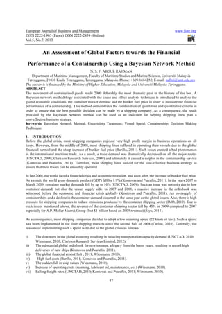
Vol.5, No.7, 2013

Figure 4: The analysis of the node “Financial Analysis” given evidence to the node “CMD=decrease”
After giving a piece of evidence to the node “CMD=decrease”, the result shows that the new posterior probability
value of the node “VS=low steaming” increases from 0.4026 to 0.6847 (Figure 4). Due to such an increase of the node
“VS=low steaming”, the posterior probability values of all nodes are significantly updated except the nodes “BFP” and
“GEC” because there is no correlation between both nodes with the node “Container Market Demand”. The idea of low
steaming has been introduced in the shipping industry since the middle of 2008 when the container market demand
slumped, the global economic recession and the sharp increase in bunker fuel price occurred. By giving evidence to the
nodes “CMD=decrease”, “GEC=recession” and “BFP=high”, it drives shipping lines to 100% reduction of vessel’s
speed from full steaming to low steaming (Figure 5). By adopting the low steaming speed, the probability values of the
node “TEC=more cost” is updated and increased from 0.5089 to 1.0000. Also, the node “SR=less” illustrates the
increase of the probability values from 0.5000 to 1.0000. Finally, this model shows that the probability value of the
goal node “FA=less profit” increases from 0.4933 to 1.0000.

Figure 5: The analysis of the node “Financial Analysis” given evidence to the nodes “BFP=high”, “GEC=recession”

and “CMD=decrease”

55

Vol.5, No.7, 2013

4. CONCLUSIONS
This paper uses a BN model for analysing the global economic conditions, the container market demand and the
bunker fuel prices in order to measure the financial performance of a containership under uncertainty. A test case has
been created with the purpose of demonstrating the general uncertain situations faced by shipping companies. The
developed model is dynamic and enables to be used in different situation based on uncertain situations faced by
shipping companies. In the real practice, shipping companies can add or drop any node or parameter based on the
uncertain situation faced by them. The models can also be applied in different service routes due to the flexibility of
dealing with uncertainty conditions. The output may be different if 1) different situations are adopted, 2) the total
number of experts is more or less than three and 3) different inputs are included.

REFERENCES
Barillo, N. (2011). Slow steaming – NOI, Federal Maritime Commission. Washington, D.C. 1-8.
Bernardo, J.M. & Smith, A.F.M. (1994). Bayesian theory. John Wiley and Sons Ltd.
Bonney, J. & Leach, P.T. (2010). Slow boat from China. Journal of Commerce, February 1, 11 (5), 10-14.
Buhuag, O., Corbett, J.J., Endresen, O., Eyring, V., Faber, J., Hanayama, S., Lee, D.S., Lee, D., Lindstad, H.,
Mjelde, A., Palsson, C., Wanquing, W., Winebrake, J.J., & Yoshida, K., (2009). Second IMO greenhouse gas study.
London: International Maritime Organization.
Cariou, P. (2010). The impact of speed reduction on liner shipping CO2 emissions. WMU, Working Paper July.
Clarkson Research Services (2009). Shipping Sector Reports: Liner Vessels. Available from:
http://www.clarksons.net.
Clarkson Research Services (2012). Containerships Deliveries 1996-2011. Clarkson Shipping Networks.
Corbett, J.J., Wang, H. & Winebrake, J.J. (2009). The effectiveness and costs of speed reductions on emissions from
international shipping. Journal of Transportation Research Part D, 14 (8), 593-598.
Curtis, F. (2009). Peak globalization: climate change, oil depletion and global trade. Journal of Ecological
Economics, 69 (2), 427-434.
Eleye-Datuba, A.G., Wall, A., Saajedi, A., & Wang, J. (2006). Enabling a powerful marine and offshore
decision-support solution through Bayesian network technique. Risk Analysis, 26 (3), 695-721.
Fagerholt, K., Laporte, G. & Norstad, I. (2009). Reducing fuel emissions by optimizing speed on shipping routes.
Journal of the Operational Research Society, 61 (3), 523-529.
Haglind, F. (2008). A review on the use of gas and steam turbine combained cycles as prime movers for large ships.
Part III: Fuels and emissions. Journal of Energy Conversion and Management, 49 (12 ), 3476-3482.
Hansen, A.F. (2000). Bayesian networks as a decision support tool in marine applications. Department of Naval
Architecture and Offshore Engineering, Technical University of Denmark.
Hayes, K. (1998). Bayesian statistical inference in ecological risk assessment. Centre for Research on Introduced
Marine Pests, Technical Report 17.
Holt, T. (2011). Quantim – a containership for the future, Engineers Australia – Sydney Division Presentation, Joint
RINA/IMarEst Technical Presentation, 2 March.
Institute of Chartered Shipbrokers (2009). Economics for sea transport and international trade. Seamanship
International Ltd.
International Maritime Organization (IMO) (2010). Annex VI of the IMO MARPOL Convention, London.
Jensen, F.V. (1996). An introduction to Bayesian networks. Springer-Verlag New York, Inc.
Jensen, F.V. (2001). Bayesian networks and decision graphs. Springer-Verlag New York, Inc.
Jensen, F.V. & Nielsen, T.D (2007). Bayesian networks and decision graphs. 2nd ed.. Springer Science and Business
Media, LCC.
Kjaerulff, U.B. & Madsen, A.L. (2005). Probabilistic networks — an introduction to bayesian networks and
influence diagrams. Aalborg University Press, Denmark.
Kontovas, C.A. & Psaraftis, H.N. (2011). The link between economy and environment in the post crisis era: lessons
learned from slow steaming. Available from: www.stt.aegean.gr/econship2011/index.php.
Korb, K.B. & Nicholson, A.E. (2003). Bayesian artificial intelligence. Chapman & Hall/CRC Press.
Neapolitan, R.E. (1990). Probabilistic reasoning in expert systems: theory and algorithms. John Wiley and Sons, Inc.
Notteboom, T.E. & Vernimmen, B. (2009). The effect of high fuel costs on liner service configuration in container
shipping. Journal of Transport Geography, 17 (5), 325-337.

56

Vol.5, No.7, 2013

Pakroo, H. (2008). Impact of slow steaming options on energy efficiency. In: Tozer, D. (2008) Container ship speed
matter. Lloyd’s Register. 49-50.
Pearl, J. (1986). Fusion, propagation and structuring in belief networks. Artificial Intelligence, 29 (3), 241-288.
Pearl, J. (1988). Probabilistic reasoning in intelligent systems: networks of plausible inference. Morgan Kaufmann
Publishers.
Percy, R., Vincent, J. & Fingas, M. (1996). Bunker ‘C’ fuel oil and the irving whale. Environment Canada,
Government of Canada, Montreal.
Shachter, R.D. (1998). Bayes-ball: The rational pastime (for determining irrelevance and requisite information in
belief networks and influence diagrams). Proceedings of the 14th Conference on Uncertainty in Artificial
Intelligence, 480-487.
Siyu, Z. (2011). Moller-Maersk staying afloat, China Daily. Available from:
http://www.chinadaily.com.cn/bizchina/2011-12/22/content_14304715.htm
Ullman, D.G. & Spiegel, B. (2006). Trade studies with uncertain information. Sixteenth Annual International
Symposium, INCOSE.
UNCTAD (2009). Review on Maritime Transport 2009. United Nations Publication.
UNCTAD (2010). Review on Maritime Transport 2010. United Nations Publication.
Waldo, J. (2009). Memphis role in the global/national transportation picture the importance of our infrastructure.
Global Insight Inc.
Wang, J. & Trbojevic, V. (2007). Design for safety of large marine and offshore engineering products. Institute of
Marine Engineering, Science and Technology.
Wiesmann, A. (2010). Slow steaming – a viable long-term option?. Wartsila Technical Journal, 2, 49-55.

Dr. Noorul Shaiful Fitri Abdul Rahman is currently affiliating with Faculty of Maritime Studies and
Marine Science, Universiti Malaysia Terengganu, Terengganu, Malaysia. His research interests include
steaming speed of the maritime transportation, decision making techniques, shipping economics and
finance, uncertainty treatment and modelling research in the maritime sector.

57

Assessing financial performance of containerships using Bayesian networks

Recommended

Recommended

More Related Content

Similar to Assessing financial performance of containerships using Bayesian networks

Similar to Assessing financial performance of containerships using Bayesian networks (20)

More from Alexander Decker

More from Alexander Decker (20)

Assessing financial performance of containerships using Bayesian networks